Material Flow in Product Assembly on a Production Line

1. Introduction to Simulation Models

Simulation models are tools used to represent and analyze complex real-world processes in mathematical or logical form. Their main advantage is the ability to test different scenarios and predict system behavior without interfering with the real environment. In manufacturing, simulations play a key role in process optimization, resource planning, and identifying potential bottlenecks. With the use of software such as Vensim, it is possible to graphically and intuitively build dynamic models, analyze material flows, and study relationships between individual components of the system.

2. Model Description

The developed simulation model presents a simplified process of product assembly on a production line, where the material flow between successive stages of production is analyzed. The model was built in the Vensim environment and includes two warehouses (Warehouse1 and Warehouse2), which supply plates and screws respectively as the basic components required for assembling product sets.

Warehouse1 starts the simulation with a stock of 100 plates, while Warehouse2 has 400 screws. Completing a set only takes place if both warehouses have sufficient components — 1 plate and 4 screws per set. The completing process is controlled by a logical variable that determines whether components can be drawn based on available resources. Then the sets are passed to the next stage – assembly, which occurs in a 120-second cycle. After assembly is complete, the finished units are sent to the final buffer — the assembly unit.

The model allows for analysis of resource consumption dynamics, completing rate, and the rhythm of final product assembly. It is useful in evaluating the efficiency of the production line and the impact of material availability on the continuity of the manufacturing process.

Component Equations:

Component 1:

Completing*Number of component1

Component 2:

Completing*Number of component2

Warehouse 1:

-Component1

Warehouse 2:

-Component2

 

Completing:

IF THEN ELSE(Warehouse1>=Number of sets*Number of component1:AND: Warehouse2>=Number of component2*Number of sets, Number of sets, 0 )

Set of components:

Completing-Assembly

Assembly:

IF THEN ELSE(Set of components>=1/Assembly time, 1/Assembly time, 0 )

Assembly unit:

Assembly

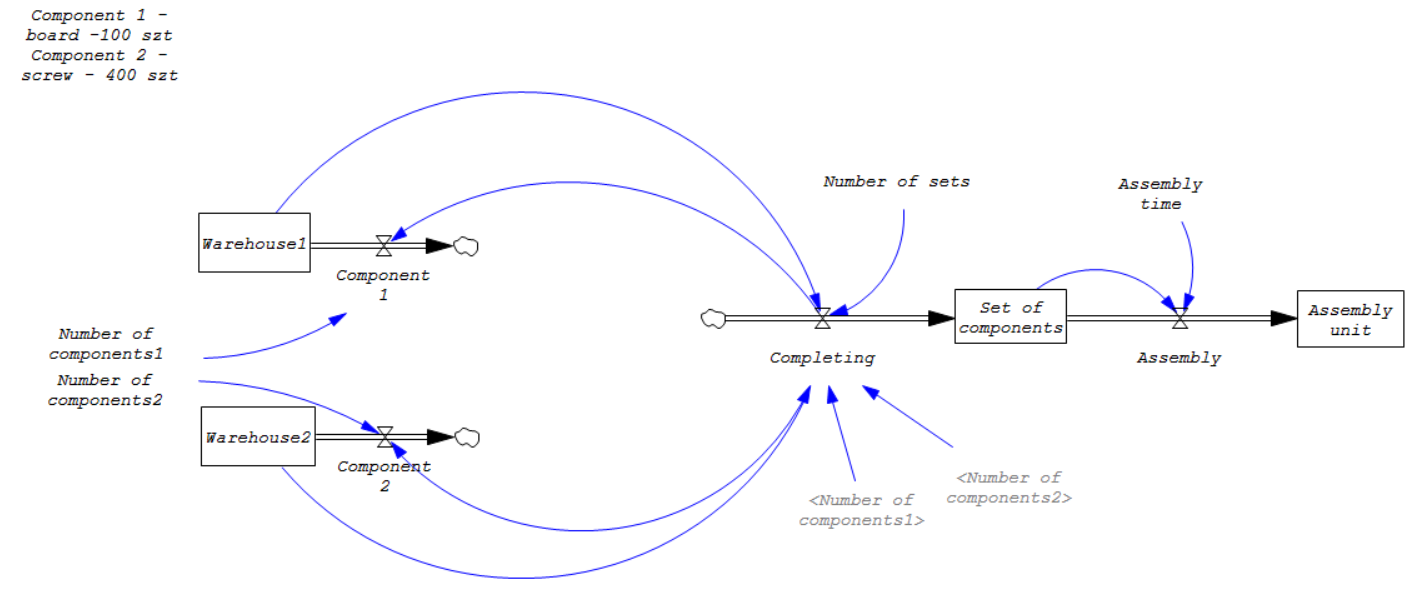
Fig. 1 Model "Material Flow in Product Assembly on a Production Line"

3. Results

Based on the attached graphs, the behavior of individual components in the simulation model over time can be analyzed: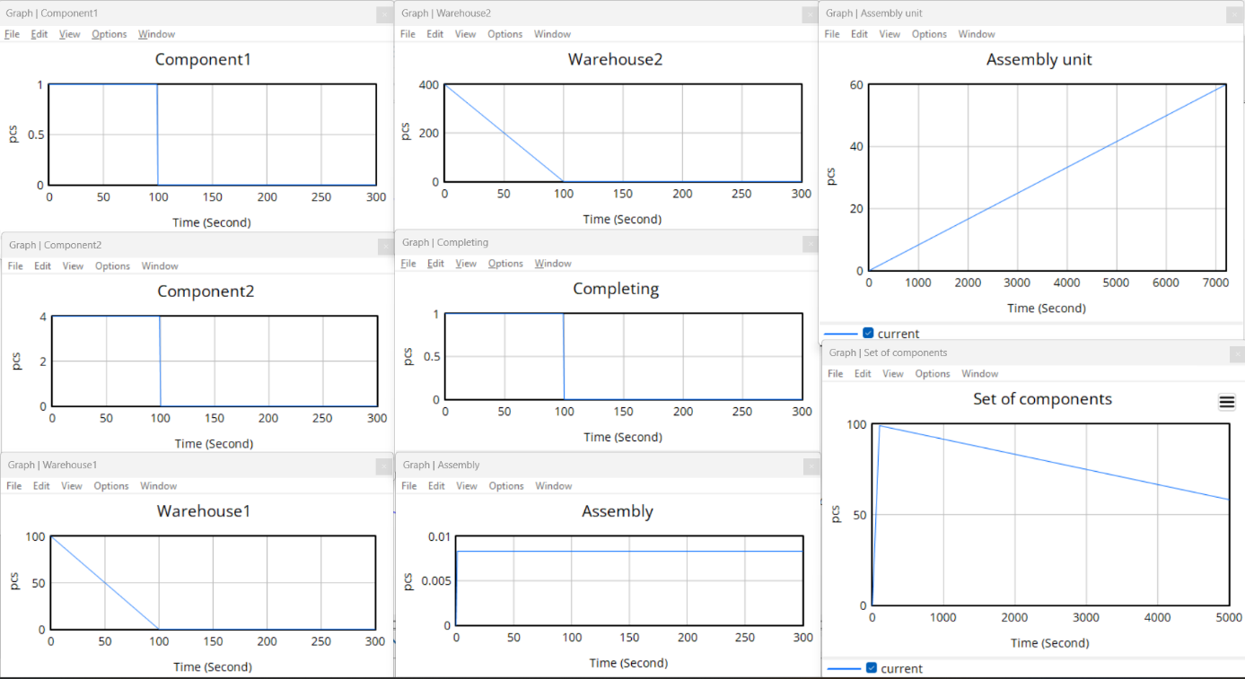

Fig. 2 Simulation Results Charts

Component 1:

The graph shows the change in the number of plates used during the simulation. It maintains a constant maximum level (value 1) from the beginning, indicating that one plate is consumed in every completing cycle. This means the logical condition in the “Completing” variable is satisfied from the start, and the process proceeds without interruption, consuming components according to the assumptions.

Component 2:

The graph shows screw consumption over time. Its value is 4, which corresponds to the requirement of four screws per set. This confirms that the completing process functions according to the model logic and uses the correct number of second-type components in each cycle.

Both graphs (Component1 and Component2) show constant consumption values throughout the simulation, indicating the process runs regularly and smoothly until one of the resources is depleted.

Warehouse1:

The graph shows a linear decline in plate stock from the initial value of 100 units. One plate is used per set. When the number of plates reaches zero, the completing process stops because the logical condition in the “Completing” variable is no longer satisfied. This halt also affects the assembly process, as seen in further stages of the model analysis.

Warehouse2:

The graph shows the time-based course of screw stock. Warehouse2 supplies Component2, four units of which are needed for one assembly set. The consumption rate is higher than in Warehouse1. The characteristic intensity of resource consumption from Warehouse2 matches the Completing graph, which shows the production of individual sets: each is prepared only when exactly 1 unit of Component1 and 4 units of Component2 are available. Therefore, maintaining sufficient stock in Warehouse2 is critical for completing — it must supply components at an adequate pace to avoid process delays.

These graphs confirm the model's correct functioning and its consistency with the mathematical assumptions. The simulation reflects actual material consumption and allows for analysis of limited resource impact on later production stages.

Assembly Unit:

The graph shows a steady increase in the number of assembled units over time. The curve is linear, indicating a regular and uninterrupted assembly process. Since the assembly takes place every 120 seconds (i.e., at a rate of 1/120 = 0.0083 units per second), the graph confirms that assembly is possible after each completing cycle. The final value (about 60 units after 7000 seconds) matches the work rate defined in the model.

Completing:

The graph shows the process of completing sets of components needed for one assembly unit. The graph cyclically reaches a value of 1, meaning one set is completed at each moment. Then it drops to zero, indicating the set was passed to assembly. This confirms that completing is a unit-based process: each product requires exactly one Component1 and four Component2s. The process synchronizes with the assembly rhythm, occurring only when resources are needed and ready for use. The regular pattern reflects efficient completing logic and no delays in component availability.

Assembly Unit:

The graph shows the number of assembled units over time. The linear, upward trend reflects the steady pace of the assembly process. The final number — around 60 units after 7000 seconds — matches the model assumptions, where each unit takes 120 seconds to assemble. The smooth graph suggests continuity and flow — resources were available in adequate amounts, and the start conditions for assembly were met throughout the simulation.

Assembly:

The graph shows the value of the variable representing the active operation of the assembly station. The constant value of 0.0083 results from the inverse of the assembly time (1/120), confirming the station remained continuously active. This graph aligns with the graph of assembled units, reinforcing the conclusion of uninterrupted assembly due to full resource availability.

Set of Components:

The graph illustrates the number of prepared sets of components used for assembly. The graph shows a linear decline — from about 100 sets initially to around 40 at the end of the simulation. This indicates systematic consumption of sets in line with the assembly rhythm. The absence of sudden drops or spikes shows that transfer to the assembly station was organized and delay-free.

4. Conclusions

The analysis of the simulation model results for material flow in the assembly process allows several important conclusions about the operation of the production system. Above all, the model shows regularity and stability, resulting from a well-designed mechanism for completing and assembly. The production process proceeds smoothly until one of the input resources is exhausted — in this case, plates from Warehouse1.

The main system constraint is component availability, which becomes evident when completing stops after the initial stock of plates is used up. The model clearly shows how the lack of a single component can halt the entire assembly process, regardless of the availability of others. This highlights the importance of maintaining appropriate warehouse levels for all components and may suggest implementing automatic stock replenishment in more advanced versions of the model.

It is also worth emphasizing that both completing and assembly proceed according to logically defined conditions. The “Completing” variable activates only when specific resource requirements are met (1 Component1 and 4 Component2s), and the process follows a unit-based logic. This structure reflects the sequential nature of production operations and allows assessment of their efficiency over time. The “Assembly” variable also remains constant, indicating consistent productivity of the assembly line based on the assumed cycle time.

This model can serve as an effective tool for supporting production planning and management, particularly in inventory control and identifying potential bottlenecks in the process. It may also be a starting point for future expansion — for instance, with new warehouses, delay times, random factors, or variable raw material availability.

In conclusion, the simulation model in its current form faithfully reflects the key aspects of material flow on a production line, and its results provide valuable insights supporting the optimization of the assembly process.