Inventory Level Management under Stochastic Demand - Michał Sokół

 

 

Simulation Modeling Project
Course: Simulation Modeling

 

Title:
„Inventory Level Management under Stochastic Demand”

 

 

 

Student name: Michał Sokół

 Student ID: 167528

 

 

1. Introduction

Effective inventory management plays a crucial role in ensuring the continuity of production and logistics processes. Under conditions of variable and stochastic demand, planning replenishment and order quantities becomes particularly challenging, and traditional forecasting methods often prove insufficient.

The aim of this project is to present a simplified model of an inventory system that incorporates stochastic demand and a dynamically changing delivery delay. The model was developed using the Vensim simulation environment and is based on the principles of system dynamics.

The theoretical framework for this work is drawn from the study by Paweł Litwin, titled "Application of the System Dynamics Method in the Analysis of Production Processes". In this work, the author demonstrates how system models can be used to represent real-world economic processes. The model developed in this project allows for the analysis of inventory behavior under uncertainty and supports drawing conclusions relevant to supply planning policies.

 

2. Model Description and Structure

The inventory system model was developed in the Vensim environment as a classic stock-and-flow model, where the central variable is the inventory level (Stock). The model assumes that in each time unit (e.g., a day or a month), the stock level changes as a result of two opposing flows: outflow (Demand, representing customer orders) and inflow (Delivery, representing incoming replenishments).

The fundamental structure of the model is based on the following difference equation describing the inventory state:

Stock(t) = Stock(t – dt) + (Delivery – Demand) × dt

where dt is the simulation time step. The variable (Stock) represents the current number of product units available in the warehouse.

The variable (Demand) is defined as stochastic customer demand, generated using the function:

Demand = RANDOM_UNIFORM(5, 15, 1)

This means that in each time unit, an integer value is randomly drawn from the range 5 to 15. The stochasticity of demand reflects market variability and introduces uncertainty into the system.

The variable (Order rate) determines the replenishment strategy. Its value is calculated as the difference between the desired inventory level (Desired stock) and the current stock (Stock), constrained by logical bounds:

Order rate = MIN(30, MAX(0, Desired stock – Stock))

The use of the MAX function prevents negative values (since a company cannot return or cancel excess inventory), while the MIN function caps the order volume, reflecting practical constraints such as logistical or budgetary limitations.

A key enhancement that adds realism to the model is the variable (Delivery delay), which determines the time required for deliveries to be fulfilled. Unlike basic models that assume a fixed delivery time, this one introduces a dynamically changing delay that depends on the current demand:

Delivery delay = 1 + 0.1 × Demand

This function models real-world situations where high demand leads to supplier bottlenecks and longer lead times. The delivery mechanism is implemented using Vensim’s built-in delay function:

Delivery = DELAY FIXED(Order rate, Delivery delay, 0)

This means that each order is delivered after a delay determined by Delivery delay, with an initial delivery volume of zero.

Additionally, the variable (Desired stock) is implemented as an interactive parameter (e.g., using a slider), allowing the user to experiment with different inventory policies and examine their impact on system behavior and the risk of stockouts.

The overall model is governed by a negative feedback loop: a drop in stock level leads to an increase in the (Order rate), which after a delay causes an increase in (Delivery), and subsequently raises the stock level. The combination of delays and randomness results in natural fluctuations and oscillations, which are typical in real-world inventory systems.

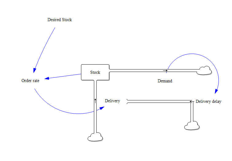
Figure 1. Stock-and-flow diagram of the inventory system

 

3. Results and Simulation Analysis

After constructing the inventory system model, a series of simulations were conducted in the Vensim environment using previously defined relationships between variables. The analysis of results allowed for the observation of inventory dynamics under stochastic demand and variable delivery lead times.

In the baseline simulation scenario, the initial stock level (Stock) was set to 100 units. In each time step, the system generated a random demand ranging from 5 to 15 units, leading to a gradual depletion of inventory. In response to declining stock levels, the system automatically triggered new orders, with the order volume determined by the variable (Order rate), constrained within the range of 0 to 30 units.

A critical factor influencing system dynamics was the variable (Delivery delay), whose value depended on the current level of demand. As demand increased, delivery times extended, reflecting real-world supply chain bottlenecks. This relationship led to growing delays and temporary stock shortages, visible in the simulation plots as drops in (Stock) and sudden spikes in (Order rate).

A characteristic behavior observed in the model was the oscillation of inventory levels—a typical feature of systems governed by delayed negative feedback loops. When stock fell below the desired level, the system increased the order rate; however, due to delivery delays, the replenishments arrived too late, causing short-term shortages. Once the deliveries started to arrive, the system accumulated excess stock, which in turn reduced the volume of subsequent orders.

An additional side effect of delivery delays and stochastic demand was the occurrence of fluctuations in the variable Order rate, which responded sharply to sudden changes in demand. The system also exhibited a degree of natural instability, which cannot be entirely eliminated but can be mitigated through proper tuning of parameters—e.g., increasing Desired stock or reducing the sensitivity of Delivery delay.

The conducted simulations demonstrated that implementing dynamic delivery delays significantly affects the stability of the inventory system. Compared to a model with a fixed delay (e.g., Delivery delay = 2), the system with demand-dependent delay exhibited greater risk of stockouts and larger inventory oscillations. On the other hand, it provided a more realistic representation of how modern supply chains behave under fluctuating demand.

Based on the observed results, the model proves to be an effective educational tool for analyzing the influence of operational parameters on the behavior of inventory systems in an uncertain and dynamically changing environment.

Simulation results for a target inventory level (Desired Stock) set to 50 units are presented below.

 

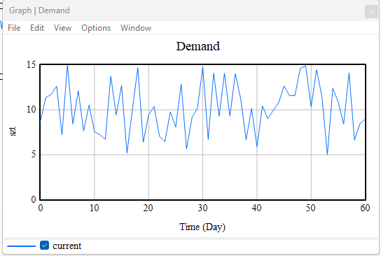
Figure 2. Demand

The graph illustrates the randomness of customer (demand)—values fluctuate within the range of approximately 5 to 15 units. This behavior reflects the use of a stochastic demand function (RANDOM_UNIFORM), which introduces uncertainty into the system.

 

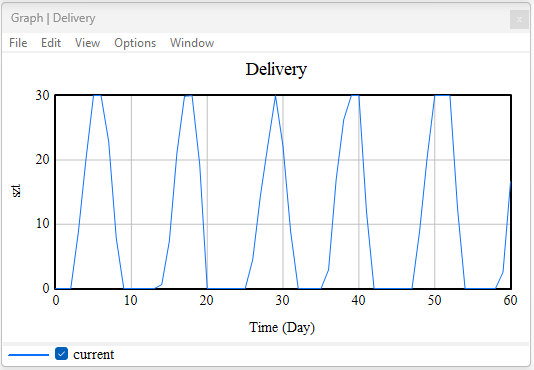
Figure 3. Delivery Delay

The (delivery delay) varies dynamically—the higher the current demand, the longer the delay. An increase in demand causes supply chain congestion, which extends delivery times and leads to further system disruptions.

 

 

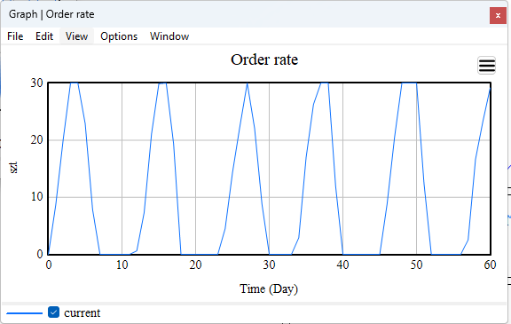
Figure 4. Order Rate

The Order rate fluctuates sharply when the stock level drops below the desired threshold. The system reacts aggressively to shortages, but due to delivery delays, the orders arrive late, resulting in additional variability.

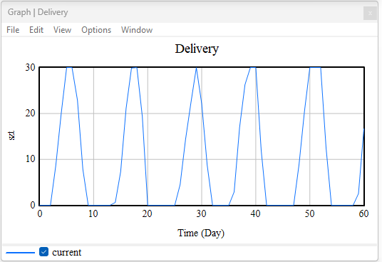
Figure 5. Delivery

Deliveries are fulfilled according to orders but arrive with a delay. Characteristic "peaks" appear shortly after increases in the (Order rate). The cycle—low stock → order increase → delayed delivery → stock replenishment → reduced orders—repeats itself over time.

Figure 6. Inventory Level (Stock)

The (Stock) variable exhibits classic oscillations typical of systems with delay and negative feedback. After reaching lower limits, the stock is replenished, but due to delays, the system constantly oscillates between shortage and surplus.

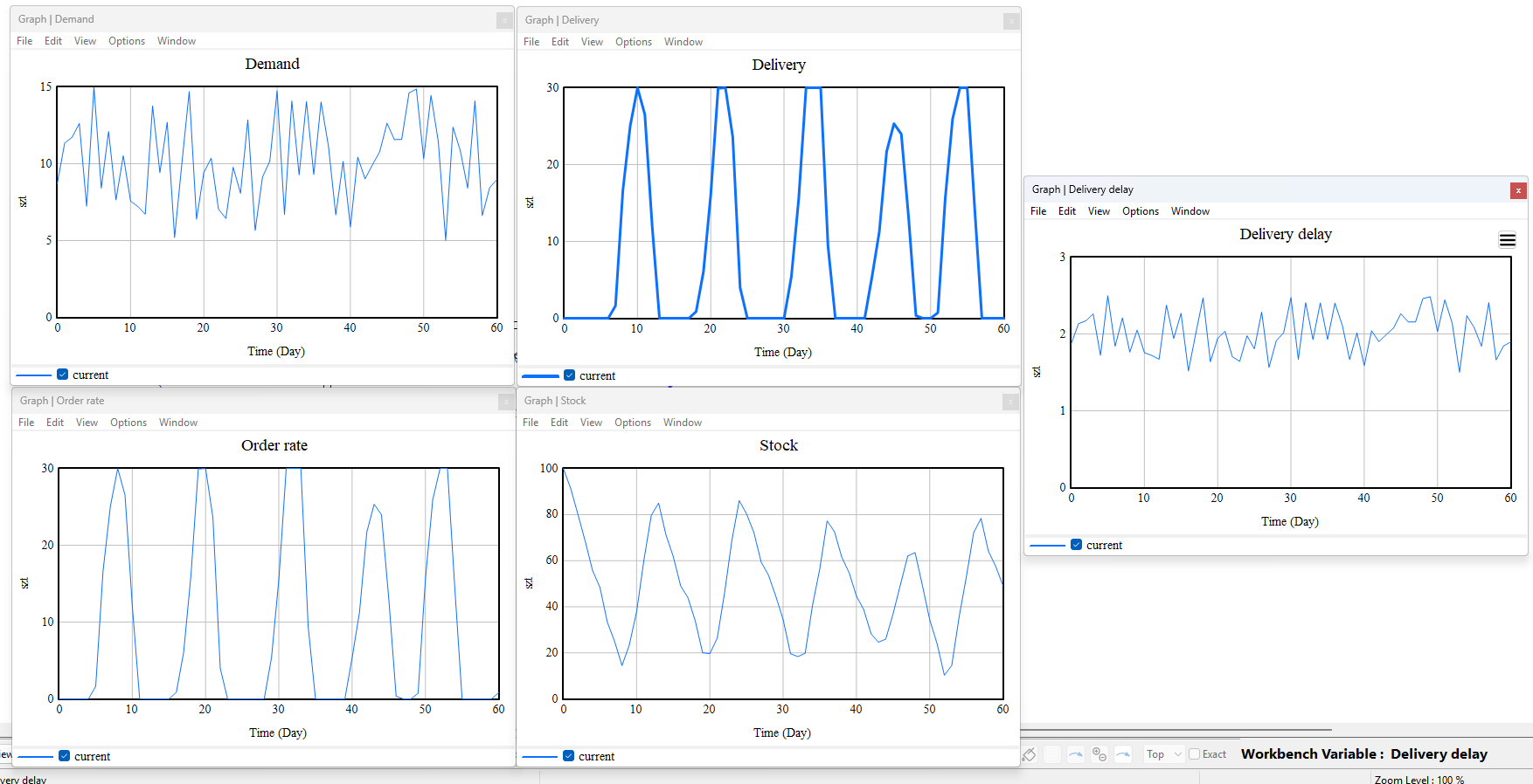
Figure 7. Simulation results for key model variables: Demand, Delivery, Delivery delay, Order rate, and Stock

 

4. Conclusions

The developed inventory system model, incorporating stochastic demand and dynamic delivery delays, enables an in-depth analysis of the relationships involved in inventory management under uncertainty. Simulations carried out in the Vensim environment demonstrated that even a simple structure based on a limited number of variables can generate complex and unpredictable system behavior.

The implementation of demand-dependent delivery delays added realism to the model and made it possible to simulate the effects of supply chain congestion. Inventory level oscillations, sudden changes in order volumes, and fluctuations in delivery times are all typical of real-world systems in which delays in response to disruptions are common.

The model also highlighted that proper tuning of system parameters—such as the (Desired stock) level or the maximum (Order rate)—is critical for maintaining system stability. Improperly selected values may lead to system instability, stockouts, or excessive inventory accumulation.

From a didactic perspective, the model provides a valuable tool for understanding the fundamental principles of system dynamics, including the role of delays, feedback loops, and randomness in shaping system behavior. It may serve as a foundation for further development, such as incorporating cost analysis, demand seasonality, or forecasting mechanisms.