Analysis of Fund Allocation in the Project

1. Introduction

Simulation models are used to represent complex real-world processes through mathematical equations and relationships between variables. Their purpose is to analyze system dynamics over time, predict behavior, and support decision-making. System simulations are particularly useful when the system is too complex to be analyzed using analytical or experimental methods – for example, in project management, economics, or logistics.
One of the popular environments for building such models is Vensim, which allows the creation of models based on flows and stocks and visualizes relationships in graphical form.

2. Model Description

The simulation model illustrates how financial resources are allocated and consumed during the implementation of a project, taking inflation into account. The central element of the model is the project budget, from which funds are allocated to three main spending categories: Salaries, Component Supply, and Operational Fees. Salary costs increase gradually and predictably, reflecting stable employment and moderate inflation impact.

Component supply costs are incurred in a stepwise manner at specific points in the project (months 6, 12, and 18), and their value increases over time, modeling price increases due to inflation and additional markups. Operational fees also grow over time, but with greater dynamics, reflecting the influence of external factors such as general inflation and variable service costs.
The model enables the analysis of total operating costs over time and identifies critical spending moments, supporting financial planning and risk management within the project.

Equations of Elements:

Operational fees:
120000*(1+(Inflation+0.02)*Time/12)

Components supply:
IF THEN ELSE(Time=6, 1e+06, IF THEN ELSE(Time=12, 1.5e+06 , IF THEN ELSE(Time=18, 2e+06 , 0 ) ) ) * (1+(Inflation+0.01)*Time/12)

Salaries:
100000*(1+(Inflation-0.01)*Time/12)

Project budget:
-Components supply - Operational fees - Salaries

Payroll costs:
Salaries

Operating costs:
Operational fees

Components:
Components supply

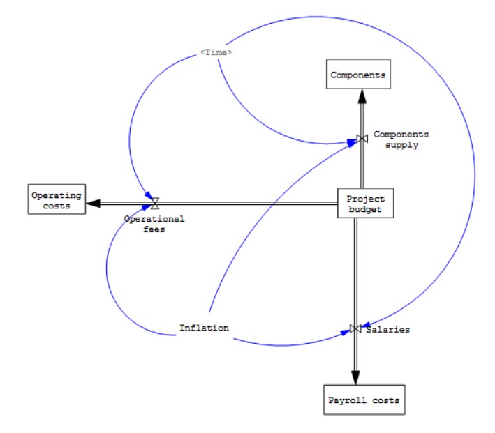
Fig. 1 Model “Analysis of Fund Allocation in the Project”

3. Results

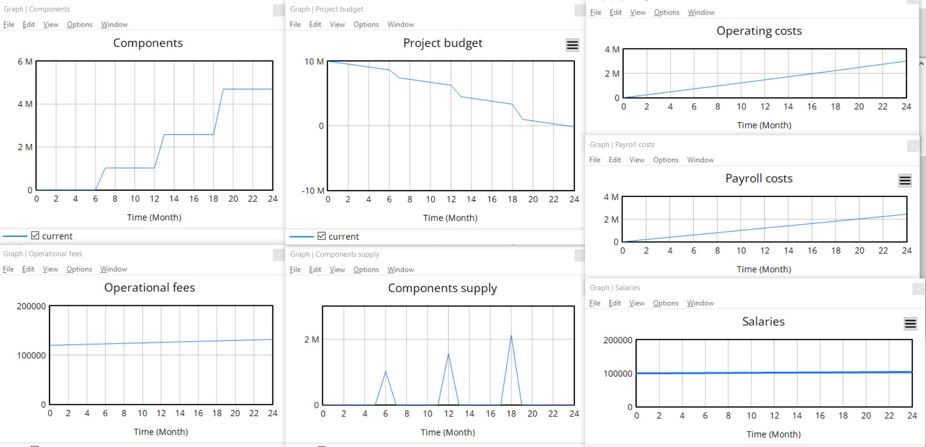
Fig. 2 Simulation Results Charts

Project Budget:

The graph illustrates the decline in the available project budget over time. The initial budget is gradually consumed by increasing operational costs, salaries, and component purchases. Sharp, sudden drops in the budget are visible in months 6, 12, and 18 – the component purchase moments – which cause significant one-time financial burdens. Between these points, the budget decreases more smoothly due to steadily increasing but even operational and salary costs. In the final phase of the project, the budget approaches zero, indicating a risk of exhaustion, especially in case of delays or unforeseen expenses.

Components:
The graph shows changes in the level of components available in the project over 24 months. This variable is characterized by stepwise value increases in months 6, 12, and 18, reflecting component deliveries according to the schedule. Each subsequent increase is higher due to the influence of inflation factored into the supply equation. Between purchases, the component level remains constant, indicating no usage or further growth during these periods. The graph clearly shows how inflation impacts the increasing cost and value of subsequent deliveries.

Components Supply:
The graph presents the stepwise nature of expenditures related to component supply in the project. These costs occur as one-time events at three distinct moments: months 6, 12, and 18. Their value increases in line with planned amounts – 1 million, 1.56 million, and 2.12 million PLN – with additional consideration of inflation increased by 0.01. The result is sharp peaks on the graph, with zero costs between these points. This modeling approach reflects real-life staged material purchases, which require prior financial resource allocation at specific project milestones.

Payroll Costs:
The graph presents a gradual increase in cumulative payroll costs over the 24 months of the project. The growth line is almost linear due to the equation that includes monthly salaries of 100,000 PLN and inflation reduced by 0.01. Assuming an inflation rate of 0.03, salary costs increase steadily – reaching approximately 1.2 million PLN after 12 months and nearly 2.5 million PLN by the end of the simulation. This indicates stable employment and predictable inflation impact on personnel expenses, facilitating budget planning in this area.

Operating Costs:
This graph shows the total operating costs of the project, which comprise three main components: salaries, operational fees, and component supply. The curve shows a clear, almost linear increase, reaching around 3 million PLN over 24 months. While some costs increase gently and regularly (such as operational fees and salaries), the curve steepens at the stepwise component purchase moments (every 6 months), significantly raising total expenditures. The graph effectively illustrates the increasing budget burden as the project progresses.

Operational Fees:
The operational fees graph shows a gradual cost increase over time, following an equation that includes inflation increased by 0.02. With default inflation at 0.03, this results in an annual increase of about 5%. The graph shows a steady rise from an initial level of 120,000 to a final value close to 132,000. The curve’s gentle slope indicates a predictable and stable cost increase in this category. Compared to salaries, operational fees have a greater impact on budget dynamics, although their growth remains moderate.

Salaries:
The graph presents the variability of salary costs on a monthly basis over two years. These values result from an equation dependent on inflation, where wage growth is adjusted for inflation reduced by 0.01. At the set inflation rate of 0.03, the effective annual salary growth is only 2%. Consequently, the graph line remains nearly flat, indicating very minimal cost changes over time – from an initial 100,000 to around 104,000 by the end of the simulation. This shows that salaries are relatively stable costs in the model.

4. Conclusions

The analysis of the simulation model results allows for several key conclusions regarding project budget management. Most importantly, the greatest financial risk is associated with sudden, stepwise expenditures on components, occurring in months 6, 12, and 18. These one-time burdens significantly reduce the available budget and may lead to its quicker depletion if not properly planned.
In contrast, salary and operational costs exhibit a predictable, gradual increase, making them easier to control and plan for. Payroll expenses are particularly stable, with minimal, nearly linear growth due to moderate inflation impact. Operational fees grow faster but also regularly, allowing their budget impact to be forecasted.
Component graphs show that stock increases occur only at delivery points, highlighting the need for close monitoring of inventory and purchase schedules.

Total operating costs increase over time, reaching around 3 million PLN after 24 months, with acceleration at component delivery points. As a result, the model accurately reflects real mechanisms of fund allocation in long-term projects, emphasizing the need for special oversight of critical moments and incorporating inflation effects in financial planning.