Inventory Level Management with Random Demand

1. Introduction

Inventory management under conditions of uncertainty and delivery delays presents a significant challenge in logistics and initial planning. To analyze the maintenance of the warehouse system, a simulation model based on a system controller was used. The model was developed in the Vensim environment, which enables graphical representation as well as practical numerical analysis. The goal of the model was to replicate the inventory replenishment process under conditions of random demand, incorporating delivery delays and attempting to maintain inventory at a specified target level.

2. Model Structure

The model represents a simplified inventory management system, which includes the following elements:

• Warehouse – Represents the current inventory level available in the system. It is a state variable that changes due to deliveries and product releases.

• Delivery – The inflow of goods into the warehouse, replenishing the inventory. It is a flow variable controlled by the difference between the expected inventory level and the current inventory level in the warehouse.

• Product Release – The outflow of goods from the warehouse in response to demand. It is a flow variable limited by the available stock in the warehouse and the current demand.

• Demand – A random input variable that determines the demand for goods in a given period. It models market uncertainty.

• Expected Inventory Level – A constant target level the system strives to maintain.

• Delivery Interval – The time interval at which deliveries to the warehouse are made.

• Market – Accumulates the amount of goods released from the warehouse that have satisfied the demand.

The model is based on the following mathematical relationships:

Warehouse:

Delivery - Product Release

 

Market:

MIN(Product Release, Demand)

Delivery:

IF THEN ELSE (MODULO( Time, Delivery Interval) = 0, Expected Inventory Level - Warehouse, 0)

Demand:

RANDOM UNIFORM(500, 1000 50)

Delivery Interval: 1

Expected Inventory Level: 1000

Product Release:

IF THEN ELSE( Warehouse > 0, MIN(Warehouse/2, Demand/2), 0)

Figure 1. Inventory Management Process Model with Random Demand

3. Simulation Results Analysis

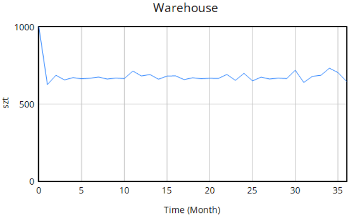
Warehouse (Inventory Level)

The graph shows the inventory level in the warehouse over time (in real-time). The available stock starts at approximately 1000 units, after which the inventory stabilizes, fluctuating around 650–750 units. These fluctuations are caused by the randomness of demand and the cyclical nature of deliveries. The chart illustrates how the inventory system maintains a balance, avoiding stockouts due to built-in system constraints that prevent inventory depletion caused by coincidental demand surges.

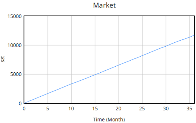
Market

The graphs show the cumulative amount of goods that have been released from the warehouse and have satisfied demand throughout the simulated period. The line on the graph is linear and increasing, indicating that demand is being met and that goods are consistently reaching the market, albeit with some delay. There are no visible drops or surges in the delivery frequency, which confirms the efficiency and stability of the system's supply process.

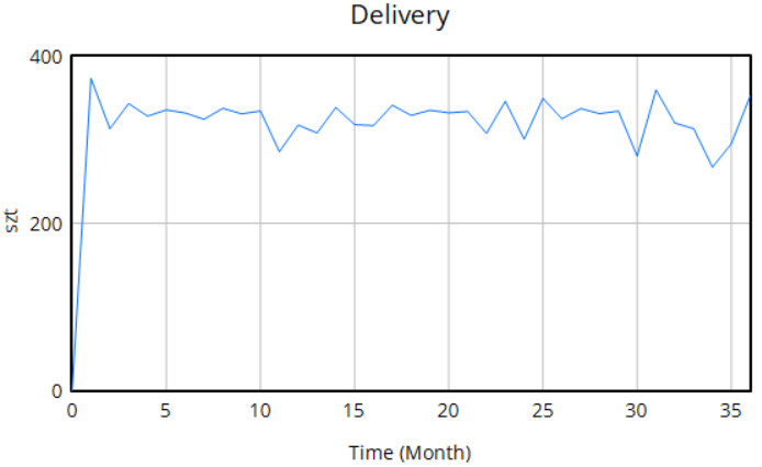
Delivery

The delivery graph shows the amount of goods regularly supplied to the warehouse. Deliveries occur every 2 months, and their volume varies depending on the current inventory level and the system's target stock level. The initial, larger delivery is intended to quickly replenish the warehouse after an early drop in inventory, after which the deliveries adjust according to actual needs.

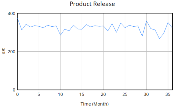
Product Release

The "Product Release" graph shows the quantity of goods leaving the warehouse. This graph closely corresponds to both demand and available inventory. Fluctuations are visible, reflecting random variations in demand, but they generally stabilize around 300–350 units. When compared with the "Demand" graph, it can be observed that the system largely meets demand, which is crucial for effective inventory management.

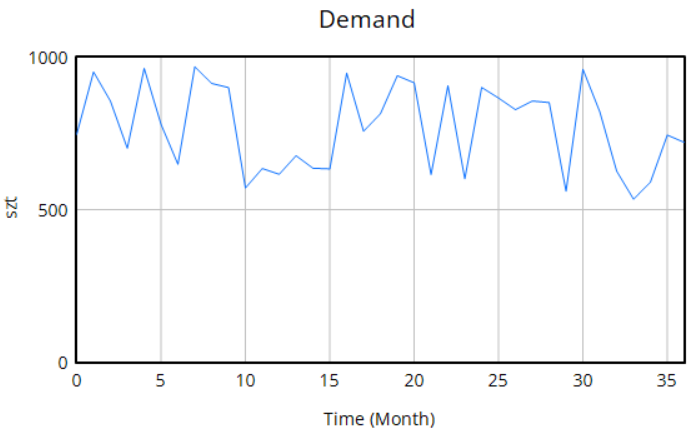
Demand

The "Demand" graph illustrates the random nature of product demand. Noticeable fluctuations occur over time, with values ranging approximately from 500 to 1000 units, in accordance with the function applied in the model. This variability highlights the dynamics of the warehouse system and the challenges that the model is designed to address.

Expected Inventory Level

The expected level is set as a constant value (1000 units), which serves as the system’s reference point for inventory control. The lack of change in this base value limits the adaptability of the inventory management strategy in real time—the model operates with a fixed decision threshold.

4. Conclusions

The conducted inventory management module with random demand in the Vensim environment provides valuable insights into system behavior, effectively replicating the stock replenishment process under controlled conditions. Despite random fluctuations, the system is capable of maintaining inventory levels in the warehouse, oscillating around a target range. This suggests that the implemented delivery policy, based on reaching the desired stock level and replenished cyclically, responds well to fluctuations and minimizes the risk of shortages.

The "Market" graph confirms that the system meets demand, which is crucial for operational continuity and customer satisfaction; no noticeable gaps are observed between product release and demand, indicating well-controlled performance. Demand, as a random variable, introduces variability throughout the system, but it is consistently met, demonstrating the model’s resilience to external disruptions.

This model serves as a solid foundation for further research in inventory management, especially in the context of changing market conditions and the trade-off between cost efficiency and service level.