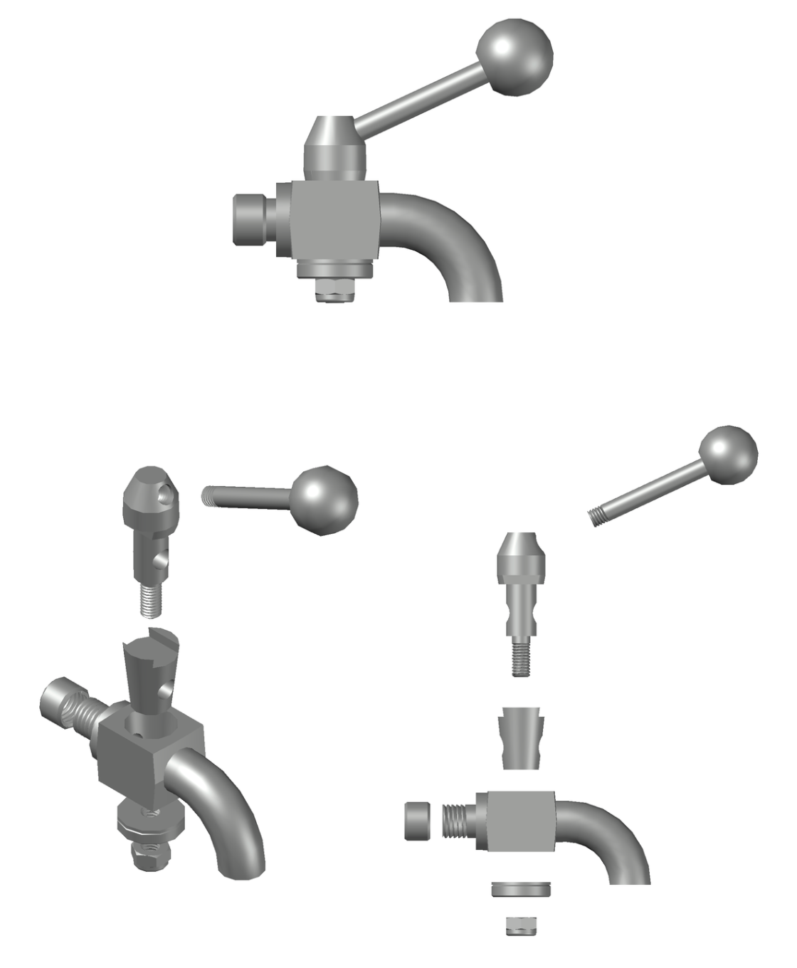
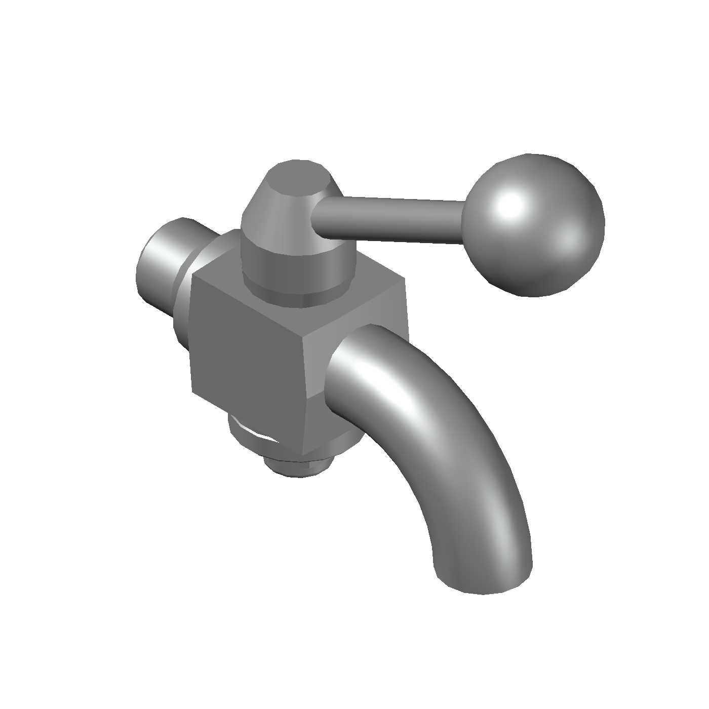
The component under study is a taper plug sampling cock (also known as a taper plug valve), designed for industrial and food-grade applications (particularly in the wine sector) thanks to the high corrosion resistance guaranteed by AISI 316 stainless steel

Below the drawings of the finished product:

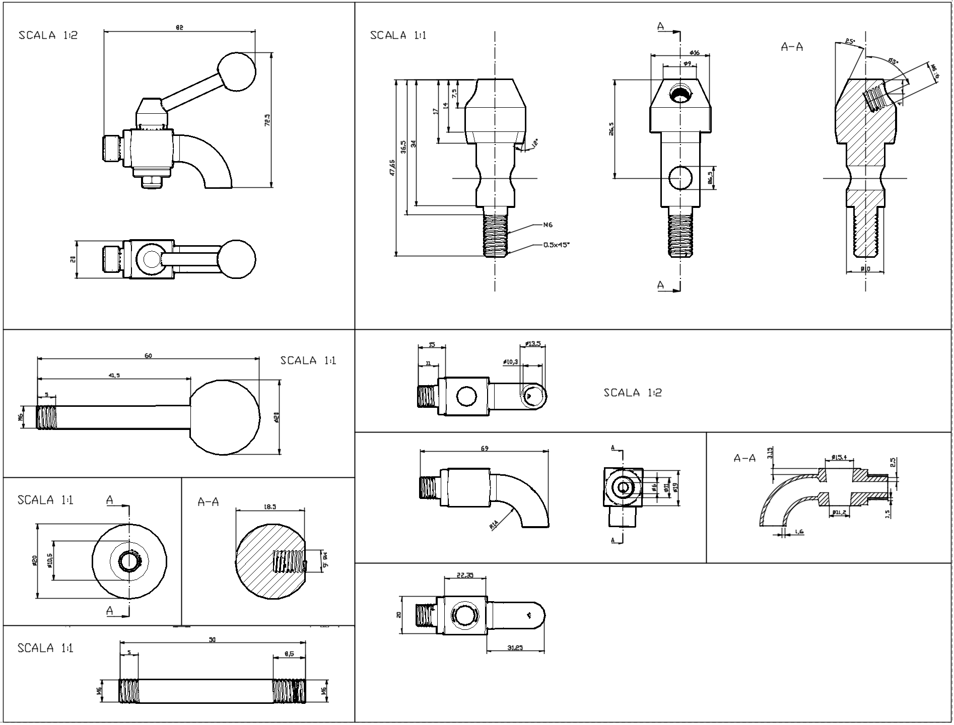
Below are the dimensions of the assembly

Foundry - Valve Body

The dimensions of the part as it leaves the foundry, ready for machining:

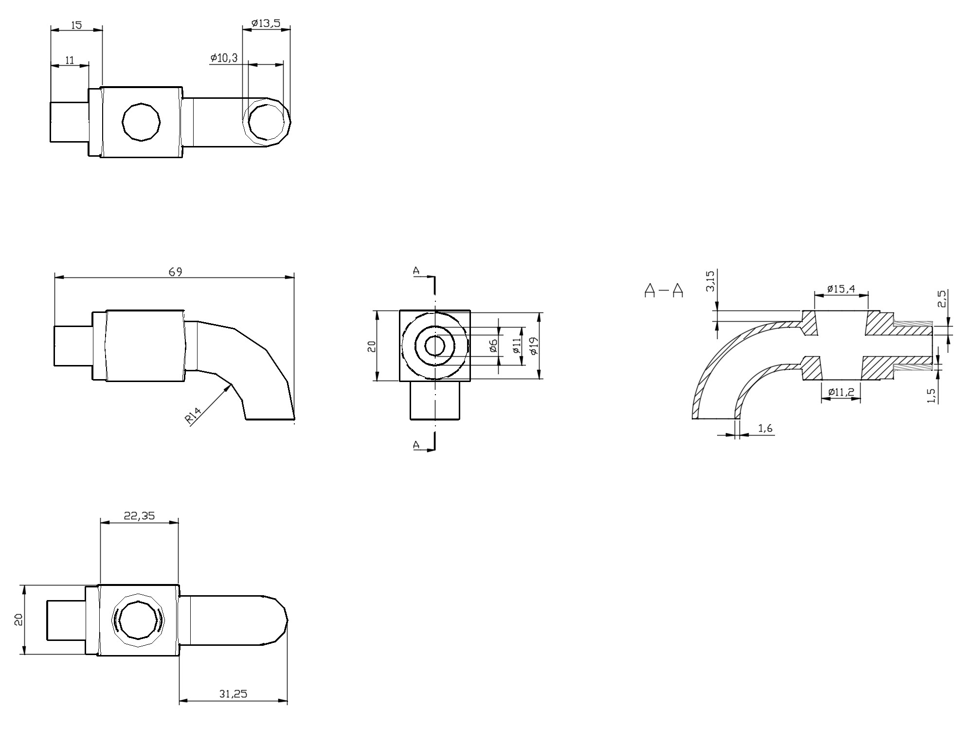
Chamfers not represented

Main characteristics of the part

For the purposes of choosing and studying the casting process, the main characteristics of the part are reported analytically:

monthly production of 500 pieces
relatively simple geometry
general machining tolerances and tolerance only on the internal conical surface for assembly equal to 0.05-0.2 mm
general surface finish Ra6 m, no special finishes
limited machining required at the interfaces (threading for installation)

Choice of process

Considering a monthly production of 500 pieces, therefore repeatable, permanent mold or pattern casting processes can be considered, which allow for:

better mechanical properties,
better quality in terms of dimensional accuracy and surface finish and
higher productivity, thanks to reduced times for molding and for solidification and cooling.

Among the permanent mold processes, we exclude die casting both by gravity and by pressure, since the alloy of which the piece is made is stainless steel: a steel die would not withstand the melting temperature of such a material, it would be necessary to resort to complex solutions such as making the die in a material with a high melting point, designing a cooling system for it and/or the use of special refractory substances with which to coat the area of the die in contact with the molten steel.

The pressure die-casting system even more so, from an economic point of view, would not be convenient due to the additional costs of the cold chamber or hot chamber machine, which are difficult to amortize given the required productivity (500 pieces/month).

The choice therefore falls on one of the techniques with a permanent pattern, in particular shell-molding.

We also exclude investment casting due to the greater slowness of the process against a higher quality not required for the piece in question.

The shell-molding process is suitable for making our part.

On the one hand, it implies an increase in costs for the purchase of machinery capable of injecting the molding material between the pattern plate and the cover and for the energy necessary to heat and polymerize the resin, furthermore the material used cannot be recovered but the waste of material is less than in sand molding, given the reduced thickness of the shells; the process is also easily automatable, the surface finish and dimensional accuracy are very good, which fall within the aforementioned tolerances, the molding material must have high flowability and be very permeable to avoid the blowhole defect. The weight of the piece is much less than the maximum limit for this process (up to 30 kg), therefore it is a good candidate to be chosen for making the part.

Choice of parting line

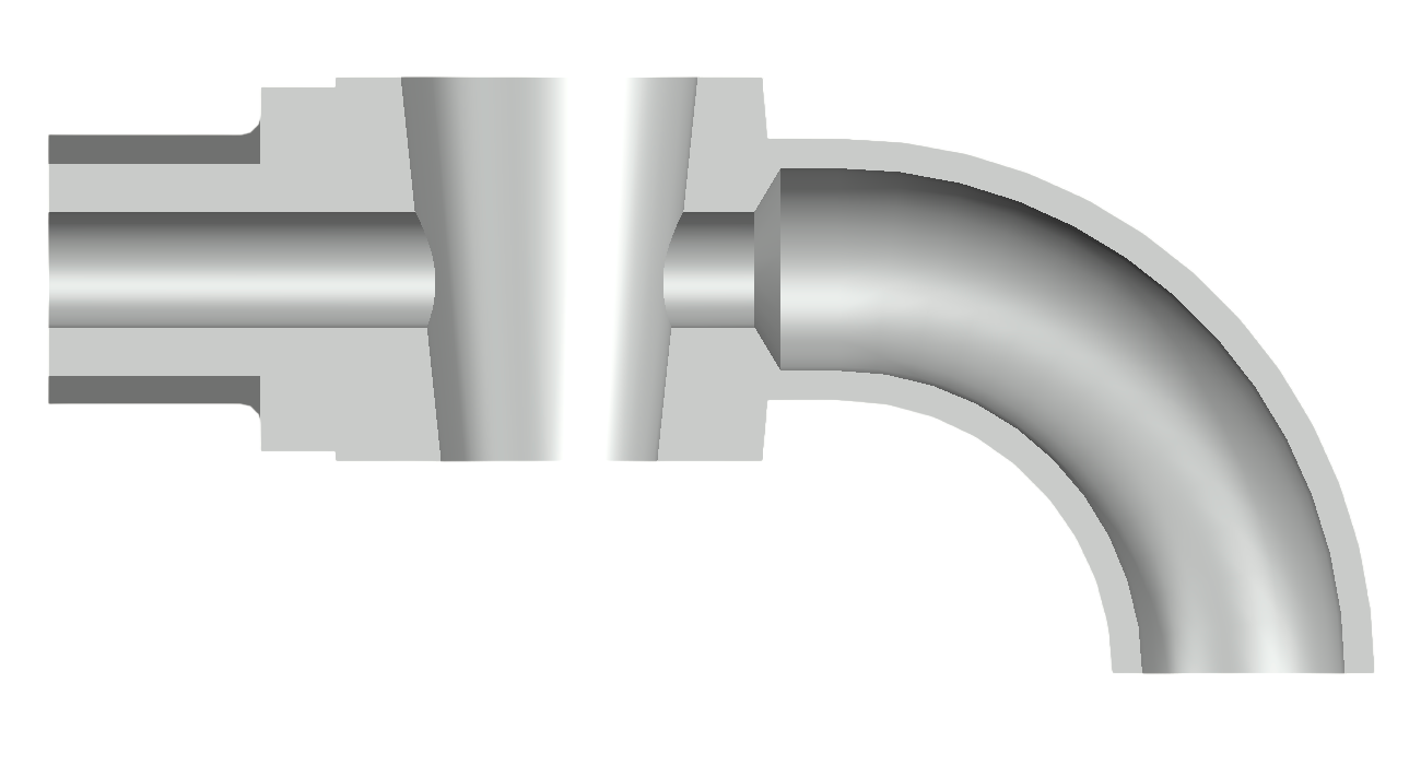
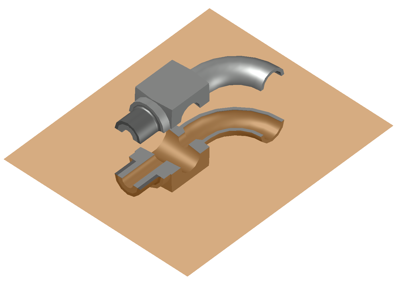
The plane of symmetry has no undercuts and is chosen as the parting line.

Machining allowances

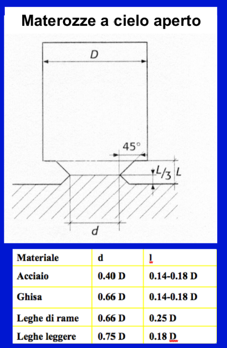
Since there are no undercuts, the machining allowance is provided only in the interface area where a thread with a relief groove will have to be executed, with the exception of the internal cavities which are generated through a core treated in the appropriate section.

Regarding the parts to be subsequently machined, the part does not have any dimension greater than 100 mm, therefore Santochi recommends a machining allowance of 1.5 mm.

Pattern simplification

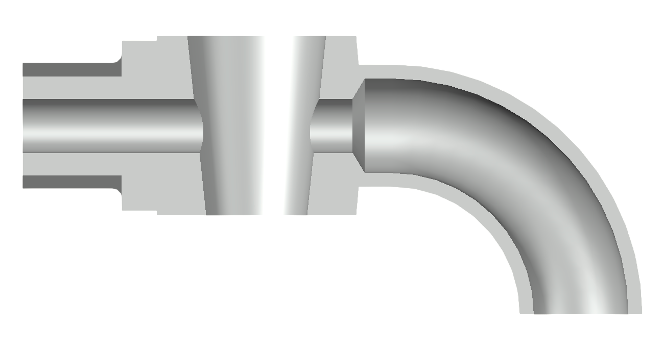
Elimination of holes

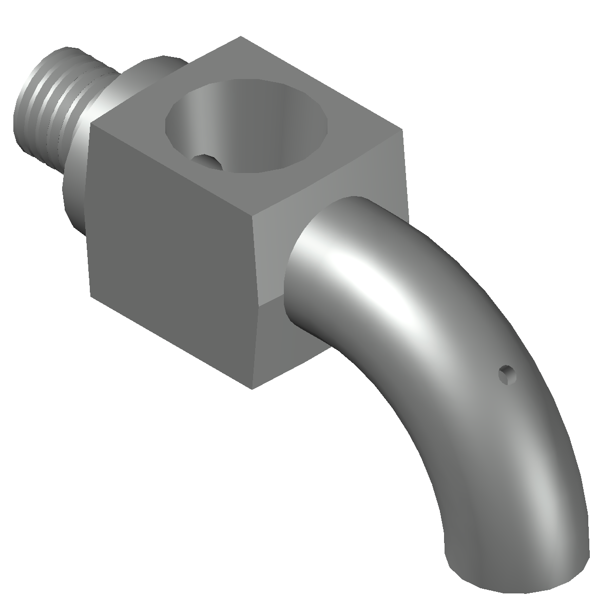
The internal cavities that are undercut are made using a core in the dedicated section.

Regarding the hole of the piece, such a thickness in a part of the shell, even if it were achievable, would make the mold fragile, with possible deformations or fractures during the solidification phase. Furthermore, if it were necessary to make a core this would entail costs and an increase in time, making it not convenient compared to making the holes a posteriori, also given the small drilling diameter.

Shrinkage

To take into account the contraction during the solidification phase and the cooling phase, the pattern plate is oversized considering the linear shrinkage of the stainless steel equal to 2 percent from the pouring temperature to room temperature.

Since it is a small steel casting, the average linear shrinkage coefficient (hereinafter ) is about 2%. Therefore the scale factor (s) is calculated as follows, taking into account the shrinkage of an edge of unit measure:

1:(1-)=s:1

s=1/(1-)=1/(1-0.02)=1.0204

Therefore, the dimensions of the pattern plate must be increased by approximately 2% compared to the nominal dimensions of the part, in order to compensate for the contraction of the material during cooling.

For reasons of speed, the dimensions of the drawing are to be intended with a shrink rule, meaning the drawing is not resized to account for shrinkage, but contains the nominal dimensions.

Draft angles

Given that we use a permanent pattern and a transitory shell, draft angles are to be provided for the molding operation (shell creation). The draft angle depends on the friction angle between the metal of the pattern plate (reduced thanks to the use of any parting powders) and the sand for shell-moulding, and corresponds to 1 degree.

The part is built by cylindrical and truncated-conical revolution surfaces which therefore do not require draft angles, and by flat surfaces perpendicular to the parting plane highlighted

Cores

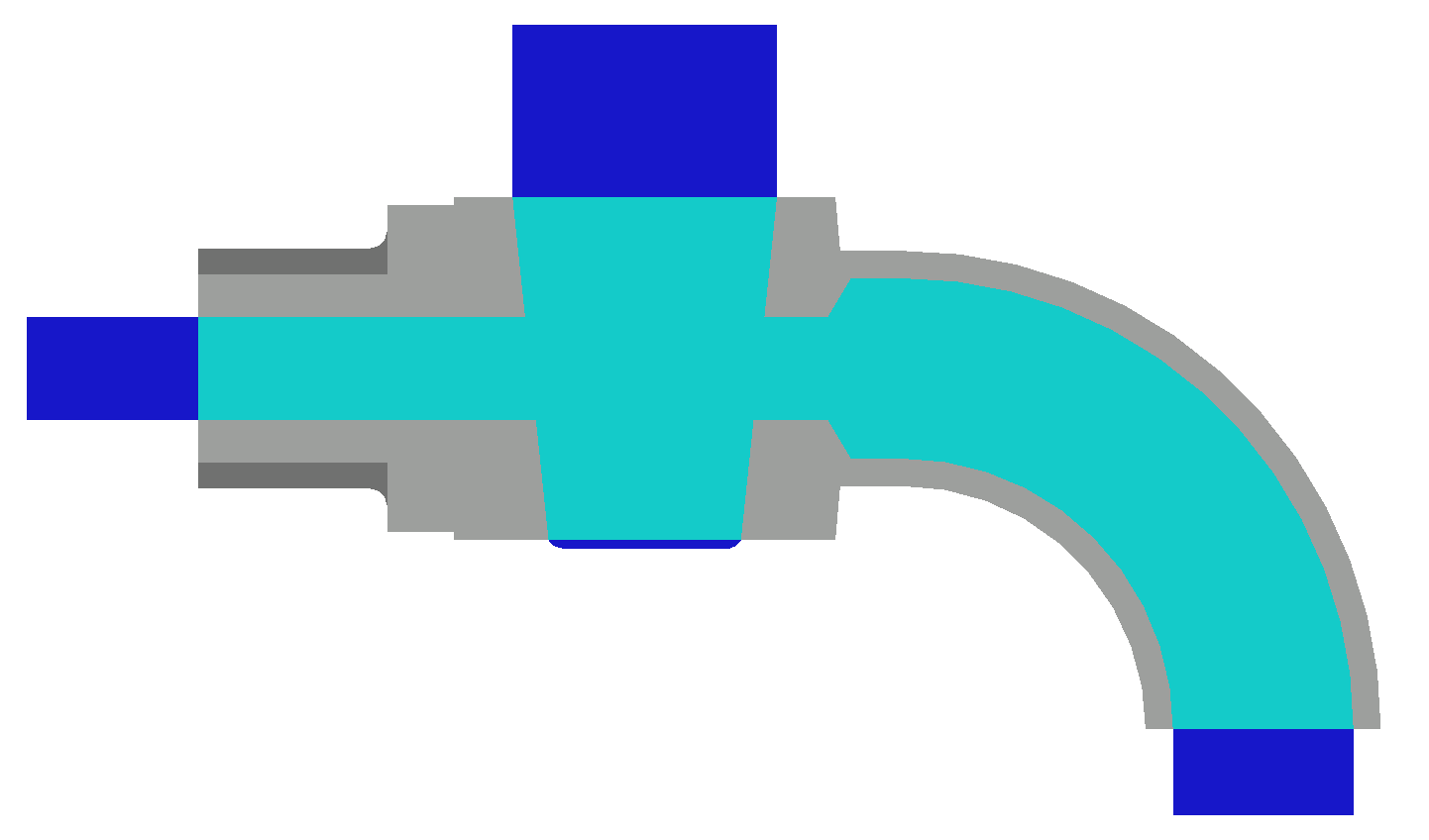
Choice of process

Considering the volumes that economically justify the use of shell-moulding, the advantages already listed remain.

Given the casting procedure chosen for the piece, the choice of the molding technique for core necessarily falls on the techniques in transitory mold. In particular, as regards the core, for homogeneity with the rest of the piece and for the observations on quality and cost-effectiveness made in the point on the choice of the process, it is decided to use the shell molding technique.

Core design

In the figure you can see the dimensioned drawings of the metal core boxes and of the core. The parting line coincides with the symmetry plan.

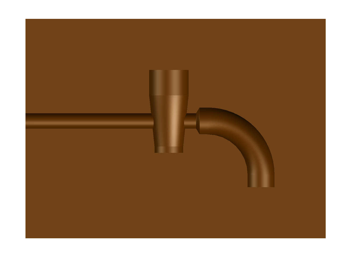
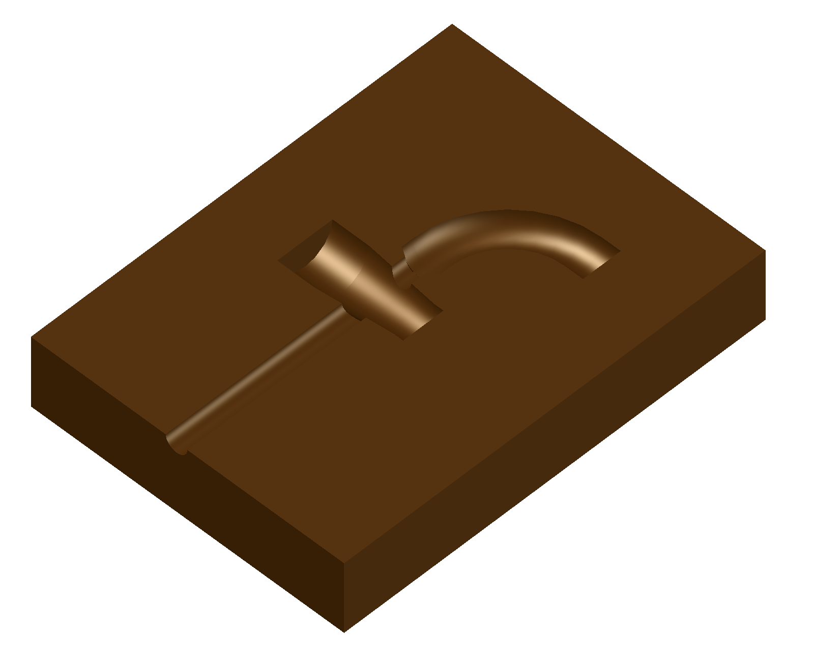
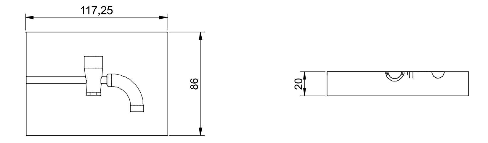
The values of the cylindrical core prints taken from company literature are 10 mm. To give maximum stability, 3 core prints are provided since the internal cavity is formed by two intersecting cavities, while a 0.5 mm diameter corer aids in the removal of the sprue at the end of the process.

Fillet radii

The fillet radii must be introduced at the corners of the mold which can be eroded by the flow of molten steel, therefore the problem exists only for the edges that generate concave angles since in the mold they will be the ones that will generate convex, protruding angles, therefore more subject to erosion.

The chamfers in the drawing of the dimensioned part and of the raw part are represented by fillet radii R=0.5 mm equal to the thickness of the machining allowance.

Directional solidification

Once the more "geometric" problems have been solved and the final shape of the raw part has been defined, to have the final drawing of the pattern plates, any components that aim to minimize foundry defects (feeders, chills, etc.) and the gating system must be designed. Between the two, the solidification of the raw part is analyzed first since the possible addition of feeders changes its geometry and weight, with a consequent increase in filling time, cost of material and energy; furthermore, the gating system can be exploited to generate hot spots and thus modify solidification.

To design any feeders, chills or other components, it is necessary to study the solidification of the raw part, to understand the direction of solidification and the critical areas and then insert the components where necessary. Lacking the gating system, it is assumed that initially the raw part is all at the same temperature. The techniques at our disposal for the study of the solidification of the casting are:

the subdivision of the casting into elementary solids and the calculation of the cooling module of the latter, to then order them and thus deduce the solidification order;
the Heuvers circle method to ensure that there are no interruptions in the flow and not to nullify the contribution of the feeder;
solidification simulation via software starting from the CAD model of the raw part.

Simplified calculation of cooling modules

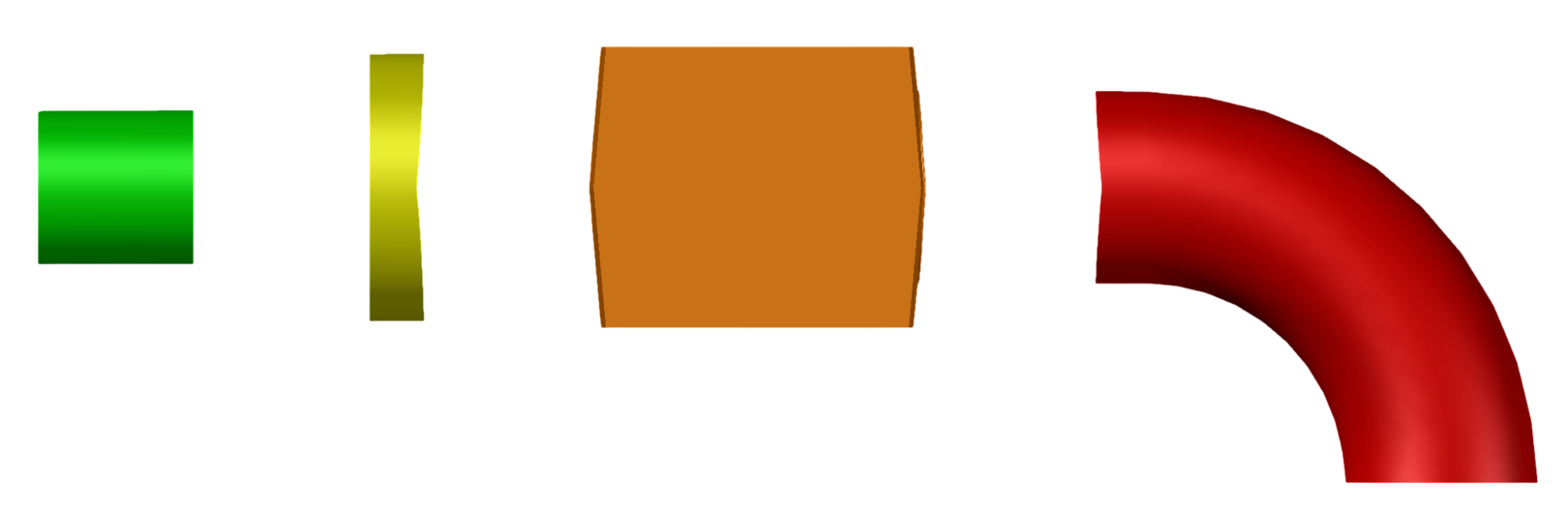
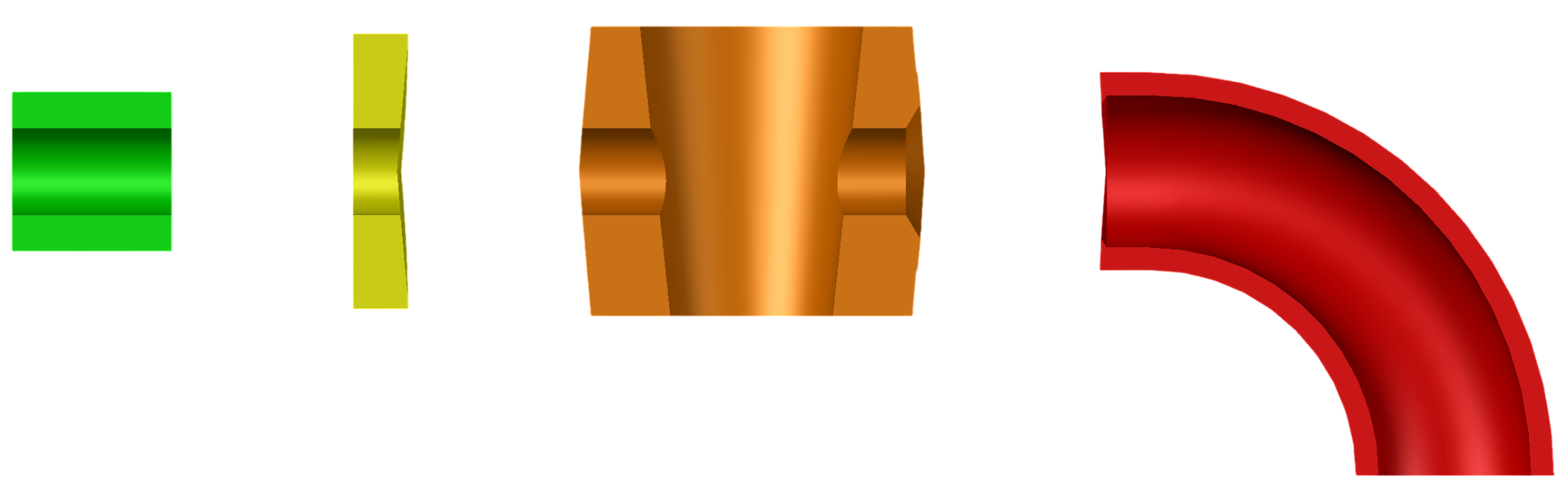
We proceed with the decomposition of the model into elementary solids. The four modules into which the part is virtually decomposed are all assimilable to a bent bar as in the estimation of the bored cylinder on Santochi, in particular:

1 (orange) cube with conical hole is assimilated to a bored cylinder; the conical hole is approximated to a cylindrical hole, with average dimension of the two bases

M1 = (S1 * S2 ) / 2 / ( S1 * S2) = (13.3 * 4.45) / 2 / (13.3 + 4.45) = 1.82 mm

the calculation is repeated considering also the thickness values at the extremes to evaluate the variability in considering the average value

M1’ = (S1 * S2 ) / 2 / ( S1 * S2) = (13.3 * 3.4) / 2 / (13.3 + 3.4) = 1.45 mm

M1’’ = (S1 * S2 ) / 2 / ( S1 * S2) = (13.3 * 5.5) / 2 / (13.3 + 5.5) = 2.15 mm

Just 16 percent variation, the average value M1 is considered sufficiently conservative, for the purpose of directional solidification.

2 (red) bent bored cylinder

M2 = (S1 * S2 ) / 2 / ( S1 * S2) = (1.6 * 39.11) / 2 / (1.6 + 39.11) = 0.76 mm

3 (green) threaded bored cylinder

M3 = (S1 * S2 ) / 2 / ( S1 * S2) = (2.5 * 11.69) / 2 / (2.5 + 11.69) = 1.02 mm

M3 with machining allowance of 1.5 mm on both sides =1.49 mm

4 (yellow) bored cylinder

M4 = (S1 * S2 ) / 2 / ( S1 * S2) = (4.5 * 6.5) / 2 / (4.5 + 6.5) = 1.23 mm

Given the presence of numerous interface surfaces, the modules could be underestimated but this applies to all four modules, therefore the effect on superficial solidification could be acceptable.

Calculation of cooling modules from CAD

To evaluate the goodness of the approximations, we proceed to the analogous calculation but in an exact manner using the CAD data, exploiting the area and volume calculation tools. At this point we proceed with the calculation of the cooling modules according to the definition:

M=V/SST

where SST is the total heat exchange surface and V is the total volume of the solid. These two data are provided by the CAD; in particular the first is obtained as the sum of the surface areas.

M1cad=1.87 mm

M2cad=0.76 mm

M3cad=1.52 mm

M4cad=1.12 mm

Therefore the solidification order of the geometries is the following: 1 3 4 2

It is therefore verified that, approximately, the solidification proceeds from the outermost parts to the most central ones, except for the threaded input module which will have to be protected by an additional feeder.

Feeder positioning

From the analysis of directional solidification based on the cooling module calculation method (cfr M1, …, M4), there is a single hot spot, therefore a single feeder is sufficient, which must be placed on component 1 with the highest cooling module.

Since M1’’ > M1’, it is decided to place the feeder on the lower side of the tap and consequently the casting will be upside down.

This positioning also improves the coverage (feeding distance) of the outlet pipe, since it is curved downwards.

Heuvers' circle method

To verify that the feeder can correctly feed the casting, the graphical verification of Heuvers' circles is performed.

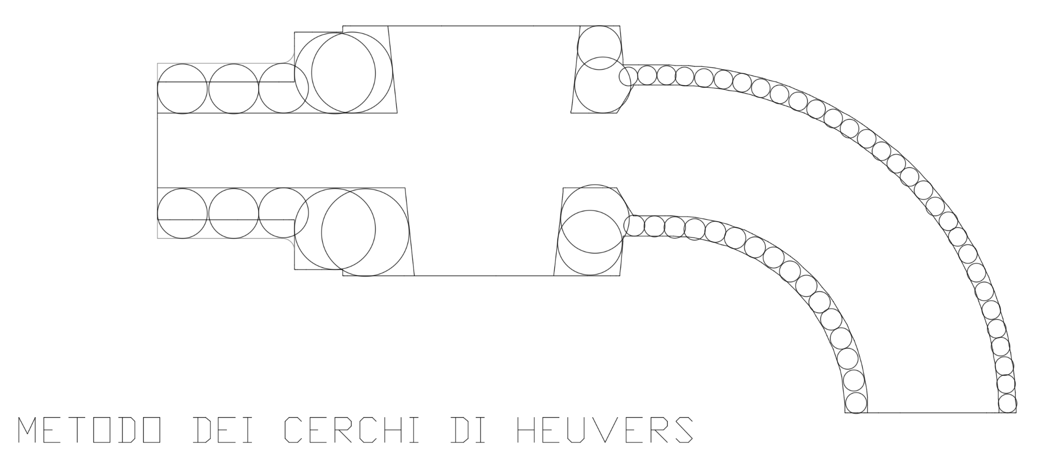
The method applied in the figure provides a positive verification on the hypothesis of feeder placement. Therefore it is not necessary to add machining allowances and then recalculate the cooling modules.

Feeder feeding distance

Since section 4 of the part (curved pipe) has a constant cross-section for its entire length, it is necessary to ensure that there are no bottlenecks that compromise the correct functioning of the feeder.

The feeding distance is:

R=k *S+2.5*S

where k is a coefficient depending on the material =3.5 and S is the wall thickness of the pipe

R1=3.5*2+2.5*2=12~mm>10~mm OK R2=3.5*1.6+2.5*1.6=9.6~mm<31.75 NOT OK

Chills

The feeder covers the inlet part while it seems insufficient for the outlet part.

Among the possible solutions, the positioning of a second feeder is discarded as it seems disproportionate to the potential benefit.

Alternatively, the possibility of increasing the thickness of the pipe was evaluated, but a design change is more onerous than a standard industrialization expedient.

The use of chills to be placed on the outlet side after forming the pattern plates is considered sufficient.

Feeder sizing

Once the solidification of the raw part has been studied, it is necessary to study how to avoid shrinkage cavities through proper sizing of the feeder.

Positioning was already discussed in the dedicated section.

First of all, the module that the feeder must have to be able to solidify last is calculated. Calling Mmax the maximum module of the part, we have:

Mm1.2* Mmax =1.2*1.87=2.244 mm

The preferred choice is open-top to utilize atmospheric pressure to pump the molten metal.

The shape of the feeder is the one that occupies the minimum volume and therefore uses less material and is easy to make. Therefore, the open-top cylindrical feeder is chosen, with H=D, which is easy to mold and is the one that, for the same module, occupies the least volume.

In Santochi:

V=1.18 D

V=179 M

M=0.18 D

At this point, the following values can also be calculated:

Dm=Mm/0.18=12.46 mm

Approximating upwards to a "rounder" value, we set Dm=13~mm. Hm=Dm=13 mm

from which: Vm=(Dm/2)2Hm=1401.75 mm3

feeder surface area, to be used later for verification with Caine's curve:Sm=DmHm+Dm2/4=663.66 mm2.

The height H=D of the feeder also determines the height of the mold and the pattern plate and will influence the length of the sprue.

Feeder neck sizing

The feeder neck sized following the practice illustrated in the text "Santochi" is shown in the figure of the raw casting.

d=0.4*Dm=5.2 mm since the feeder will be bored due to the presence of the core, the neck will have the shape of a circular ring instead of a circle with an equivalent cross-section. The internal diameter of the circular ring coincides with that of the hole, i.e., 11.2 mm. the external diameter of the circular ring measures dm=dm2+15.42=16.15 mm

Lm=0.17*Dm=2.2~mm

The figure of the raw casting arises from all calculations and represents dimensions of the feeder and neck, gating system, and part with machining allowances and draft angles and fillet radii.

Feeder verification using Caine's method

It must now be verified that the feeder is large enough to provide the metal necessary to avoid the formation of shrinkage cavities. To do this, we use Caine's formula/diagram.

The figure shows the feeder sized in the previous paragraph which is validated using the following diagram parameters:

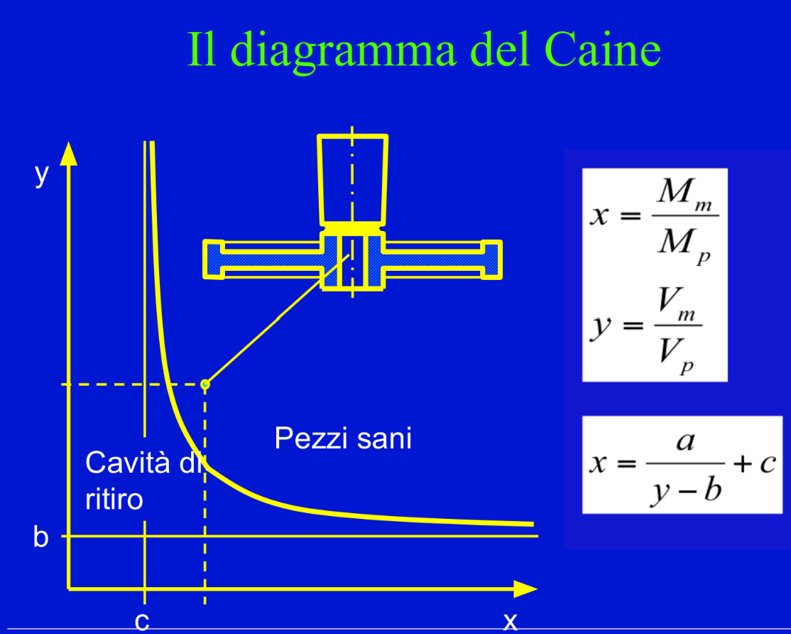
To apply it, it is sufficient to follow the algorithm on page 136 of Santochi. It is therefore necessary to define the parameters to be inserted. The parameters relative to Caine's curve are:

a=0.1 which is a fixed value;
b = 8% since the steel in question is an alloy steel;
c=1 ratio between the heat transfer coefficient of the feeder molding material and the same coefficient for the part molding material (c=1 in the majority of cases; c=0.70.8 for insulated feeders);

For what was said before, an open-top feeder is chosen and, for ease of molding, cylindrical in shape.

The values provided by the CAD software are:

Vp=9850.0272 mm3

Sp=6837.1936 mm2

Mm is the cooling module of the feeder =2.24 mm

Mp is the cooling module of the last section to be protected =1.87 mm

Vm is the volume of the feeder calculated in the specific feeder section

Vp is the volume of the entire part =9850.0272 mm3

For the estimation, the specific Matlab code shown below was developed.

clear; clc; close all;

% --- 1. MATERIAL PARAMETERS (Caine's Equation) ---

% The formula is: X = a / (Y - b) + c

% Below are the classic values for STEEL:

a = 0.1;

b = 0.08;

c = 1.00;

% --- 2. DATA OF YOUR CASTING AND FEEDER ---

V_getto = 9.84; % Volume of the casting [cm³]

A_getto = 68.37; % Surface area of the casting [cm²]

V_mat = 1.4; % Volume of the feeder [cm³]

A_mat = 6.64; % Surface area of the feeder [cm²]

% Calculation of Thermal Modules (M = V / A)

M_getto = V_getto / A_getto;

M_mat = V_mat / A_mat;

% Calculation of coordinates for the point on the diagram

X_punto = M_mat / M_getto; % Module ratio (X-axis)

Y_punto = V_mat / V_getto; % Volume ratio (Y-axis)

% --- 3. GENERATION OF CAINE'S LIMIT CURVE ---

% The volumetric ratio Y must be strictly greater than the lower limit 'b'

Y_curva = linspace(b + 0.01, 1.5, 500);

X_curva = a ./ (Y_curva - b) + c;

% --- 4. PLOTTING THE DIAGRAM ---

figure('Color', 'w', 'Name', 'Diagramma di Caine');

hold on; grid on; box on;

% Defect area (under the curve) and soundness (above)

% For graphic reasons we create a patch for the sound zone

fill([X_curva, max(X_curva), max(X_curva)], [Y_curva, max(Y_curva), min(Y_curva)], ...

[0.85 0.95 0.85], 'FaceAlpha', 0.5, 'EdgeColor', 'none', 'DisplayName', 'Sound Zone (Good Part)');

% Plot of the limit curve

plot(X_curva, Y_curva, 'r-', 'LineWidth', 2.5, 'DisplayName', 'Caine''s Limit Curve');

% Plot of the point for the casting under examination

plot(X_punto, Y_punto, 'ko', 'MarkerFaceColor', 'y', 'MarkerSize', 10, ...

'LineWidth', 1.5, 'DisplayName', 'Casting under Examination');

% --- 5. AXIS CONFIGURATION AND LABELS ---

xlabel('Module Ratio X = M_{mat} / M_{getto}', 'FontSize', 11, 'FontWeight', 'bold');

ylabel('Volume Ratio Y = V_{mat} / V_{getto}', 'FontSize', 11, 'FontWeight', 'bold');

title('CAINE''S DIAGRAM', 'FontSize', 14, 'FontWeight', 'bold');

% Setting axis limits for a better view

xlim([0.5, 2.5]);

ylim([0, 1.5]);

% Adding legend and graphic notes

legend('Location', 'northeast');

% Mathematical check of part soundness

X_limite = a / (Y_punto - b) + c;

if Y_punto > b && X_punto > X_limite

text(X_punto + 0.05, Y_punto, ' CHECK OK: SOUND PART', 'Color', [0 0.5 0], 'FontWeight', 'bold');

else

text(X_punto + 0.05, Y_punto, 'WARNING: SHRINKAGE DEFECT', 'Color', [0.7 0 0], 'FontWeight', 'bold');

end

hold off;

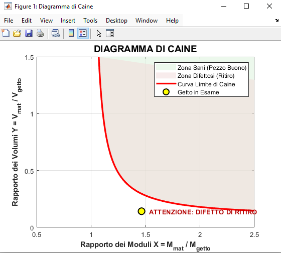
Verification with Caine's diagram shows that the feeder does not have sufficient volume to feed the shrinkage of the entire part.

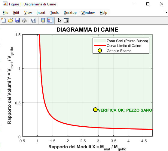
Therefore, we proceed to increase its height to 1.5*Dm instead of 1 so as to leave the sizing of the feeder neck unchanged.

Hm’=19.5 mm

Dm = 13 mm

Vm’=3882.41mm3

Sm’=929.13 mm3

Pattern plate dimensions

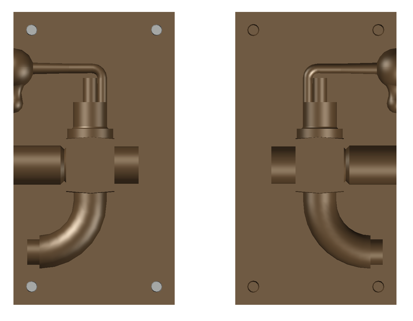
The minimum height of the pattern plate must contain the feeder and the neck and the part above the part plus a height below the part of about 15 mm.

Hm=19.5 mm and Lm=2.2 mm

resulting in 55 mm.

This value will be used to dimension the gating system.

The width is equal to the overall dimension plus an allowance of 15 mm on both sides which corresponds to 100 mm.

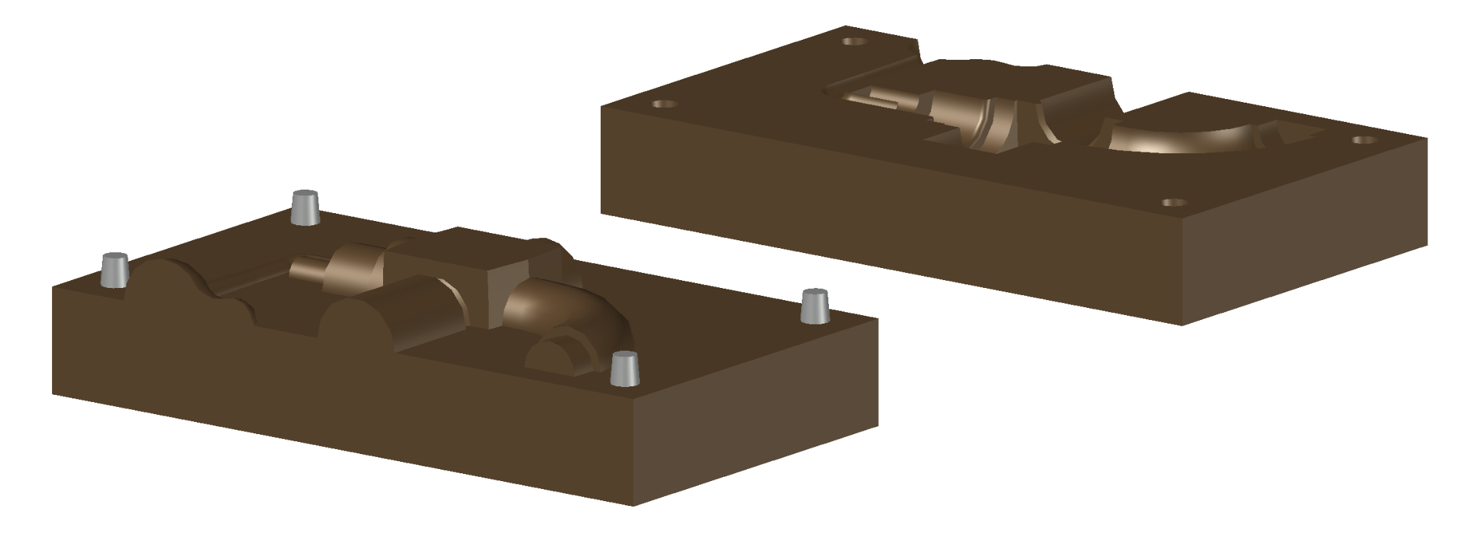
The thickness of the plate will be equal to 10 mm. pattern plate drawing

Gating system

The aspects to pay attention to in the design of the gating system are listed below:

rapid filling to avoid early solidification;
avoid high velocities;
avoid air entrapment;
block slags;
favorable thermal gradient for directional solidification;
avoid long paths, especially in thin areas.

First of all, you have to choose the type of gating system and indicate the ingates. Since the casting is small, to obtain a favorable thermal gradient, it is sufficient to use a single ingate. For aesthetic reasons, given that the removal of the ingates can leave visible marks on the surface, the outlet side is excluded, which would be preferable for the problems already outlined regarding the feeding distance of the single feeder.

The point chosen in an inconspicuous area, for aesthetic reasons, is shown in the figure.

At this point, the type of gating system must be defined: from the bottom up, from the top or side. For ease of molding, also considering that the shell-molding process was chosen, it is decidedly convenient that the gating system is made along the parting line, therefore the parting line will be vertical.

Placing the sprue in the symmetry and parting plane, there are no constraints on position due to undercut issues.

Sprue

Applying the formulas of Dietert and Nielsen proposed on Santochi

The density of the steel used is 8.0 kg/dm3

Therefore:

Vtot=Vpezzo+Vm=9841.0272 mm3+1401.75 mm3=11251.77 mm3 G=Vtot=8.0 kg/dm30.0112 dm3=0.090 kg

We now calculate the filling time T, using the following formula:

Td=3.2G=0.96 s

considering that the thicknesses b are between 1.5 and 2 mm, repeating the calculation with Nielsen's formula gives:

Tn=3.2bG0.4=2.4 s

the mass flow rate kd and kn calculated respectively with the two formulas: kd=G/Tn=0.0937 kg/s

kn=G/Td=0.0375 kg/s

At this point, the area of the sprue cross-section can be sized, using the formula: S=k/(vel*)

vel is the approximate velocity of the fluid in the section channel, neglecting the pressure drops in the sprue, and is calculated as follows:

considering the dimensions of the pattern plate, the height of the sprue which includes the curvature of the integrated ingate is derived from the height of the pattern plate to the entry point represented in the figure and is equal to:

hc=38.7 mm

vel=2ghc=0.87~m/s

Sd=13.46~mm2 which corresponds to a diameter of 4.14 mm

Sn=5.39~mm2 which corresponds to a diameter of 2.6 mm

Since the height of the free surface below the thread corresponds to about 2.5 mm due to the presence of the machining allowance, the remaining thickness of the order of a millimeter is insufficient to guarantee adequate shell strength. Therefore, it is decided to move the entry point to the tap inlet, exploiting the increased section due to the presence of the machining allowance necessary for subsequent processing, which corresponds to a total thickness of 4 mm.

Setting an ingate diameter equal to 4 mm, the section is 12.56 mm2 which is between the two values Sd and Sn previously calculated.

Since there is only one feeder neck, there is no runner and the section of the feeder neck remains constant. To maintain pressurized flow, the channel is sized following the parabolic law with acceleration due to gravity (ratio between sections inversely proportional to the square root of the heights).

As for the sprue, the textbook Kalpakjian reports that, to avoid air entrapment, the areas of the sections at any two points should follow the law:

A1/A2=h2/h1

For practicality of manufacturing, instead of literally following this (parabolic) law, it is made in a conical shape that still prevents air entrapment at the entrance of the runner, ending with a circular axis section (ingate) of constant section that acts as a choke to keep the flow continuous.

The section is circular for mold release reasons (the parting line is vertical) and manufacturing simplicity. The runner is absent since there is only one ingate. Therefore, the section of the final part of the sprue and of the ingate is constant.

Ingate

The diameter of the ingate is equal to that of the final section of the sprue. It is preceded by a filter. The presence of a slag trap is considered ineffective.

Pouring basin

For the pouring basin, the classic system with two depressions is chosen, one of which receives the beginning of the sprue and where the first slag filter is positioned. The double basin also serves to zero the velocity of the alloy falling from the crucible to respect the design flow velocity at the end of the sprue and thus avoid the risk of turbulence and mold erosion.

The casting is therefore finally the one in the raw casting figure.

Solidification time

According to Chvorinov's rule, with Mp=Vtot/Stot=16607.7268/9722.6078, given a coefficient C equal to 65-70 (for cast irons), with n=2, a time T=1.95 s results.

The values of Vtot and Stot were provided by CAD, therefore they are exact but also considering internal surfaces that have reduced exchange.

Figure of the raw casting

From the calculations performed in the previous sections, the dimensioned geometry of the casting shown in the figure is obtained, where the following are represented: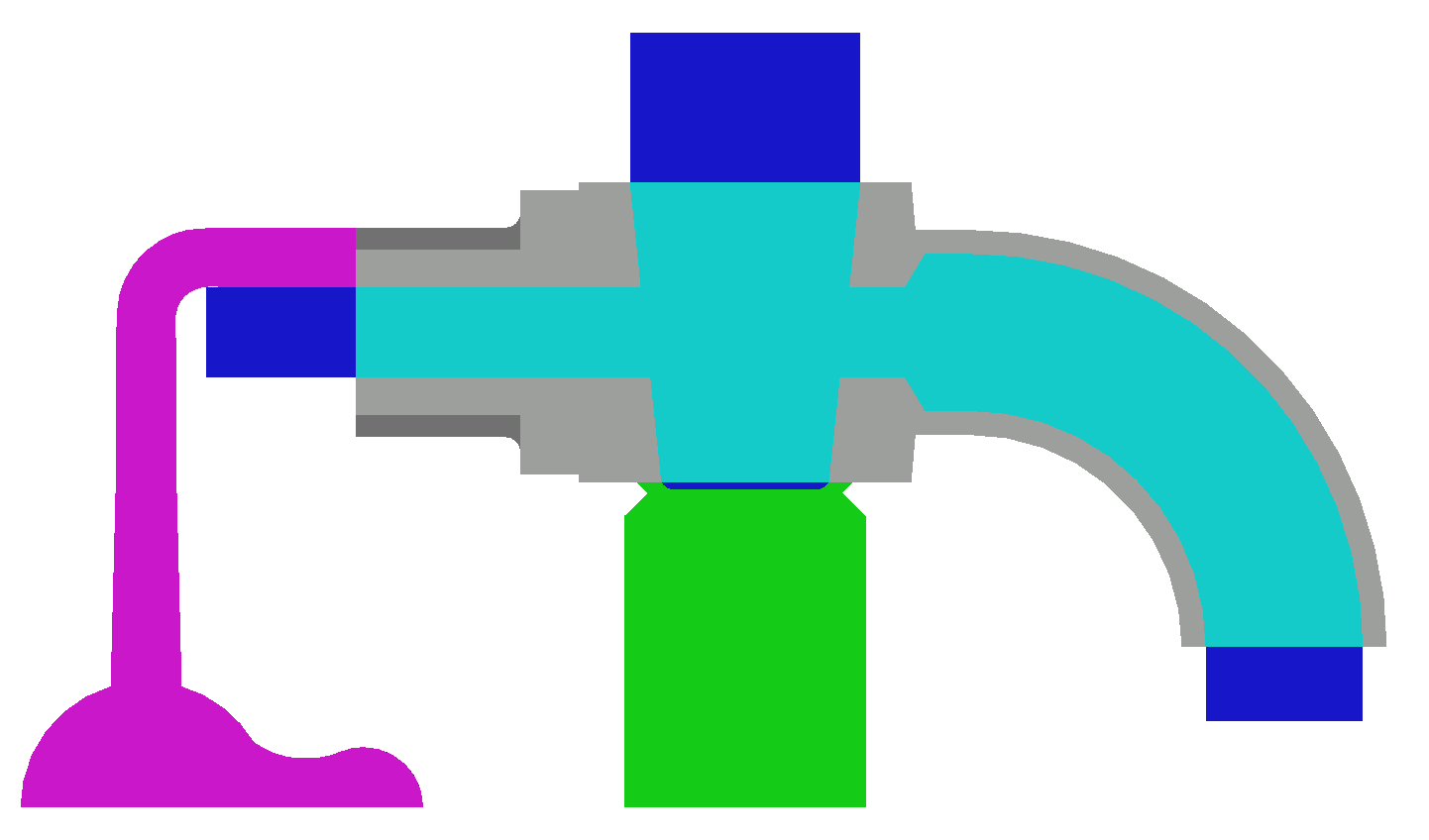

Subsequent treatments

Once the casting has cooled, the removal of the feeder and the sprue and the removal of any flashes that may have formed along the parting lines or on the contact edges between pattern and core are planned.

Simulation with SolidCast

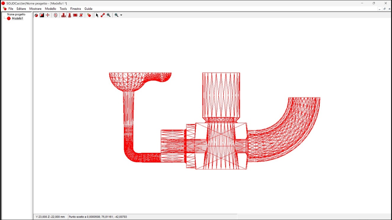
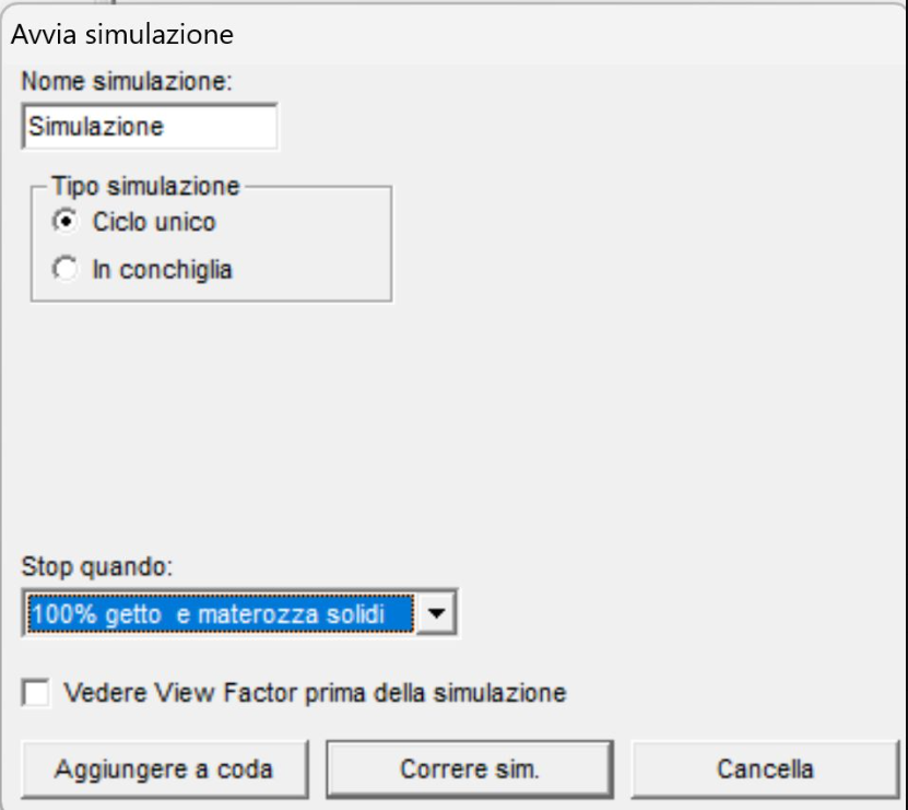
To verify the correctness of the studies carried out and to have more precise and reliable results, a solidification simulation can be performed using foundry software. After long and unsuccessful attempts with InspireCast, we fell back on the other of the two available simulation software, Finite Solution's SolidCast, version 8.2. On the downside, this program does not allow casting simulation. The part was imported in STL format already including the gating system and the feeder, so it was not possible to diversify the feeder behavior independently. Then rotating it in the direction of gravity.

After importing the CAD model of the raw part as obtained at the end of the previous point, before running the simulation it is necessary to set some parameters:

Stainless steel AISI 316 is chosen as the casting material. A shell with a thickness of 25 mm of Silica Sand material was set. Both materials are already available in the basic database.
The recommended initial temperature is chosen, i.e, 100 K above the liquidus temperature, the latter being 1371 K for the considered steel.
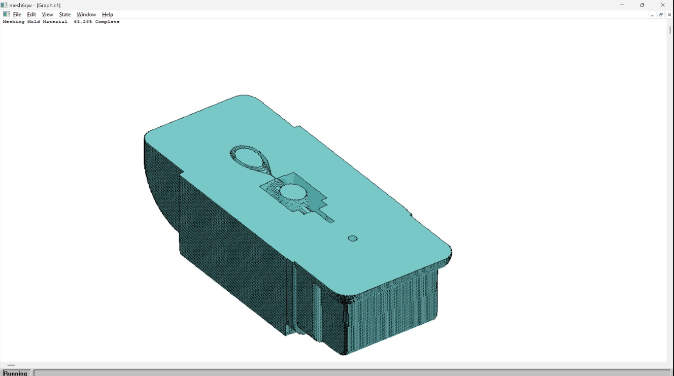
Having chosen the shell molding process, it is possible to create a shell of constant thickness around the imported model.

The program also allows multiple castings, but since it is a disposable mold, a single casting is set. The program also allows setting the shell open in correspondence with the sprue, therefore the pouring basin and the external surface of the feeder are correctly exposed to the outside.

At this point, the solidification analysis is performed, which starts from the casting in a molten state and at the same temperature, as desired. The chosen accuracy is a mesh with 1 million elements, for the rest the parameters suggested by the software are kept. A wide range of results is thus obtained, however, only the most useful ones for our purposes are reported below.

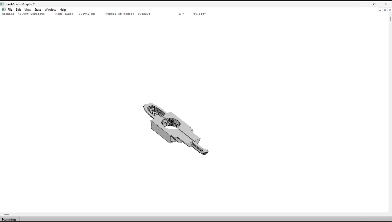
One of the most important results is certainly the video that shows over time the evolution of the "Solid Fraction" parameter in the various parts of the casting, since this is what illustrates how solidification actually occurs. As the maximum value represented for the Solid Fraction, 0.80 is chosen: it can be considered that at this point the area is almost completely solidified and the transition to complete solidification should not present criticalities.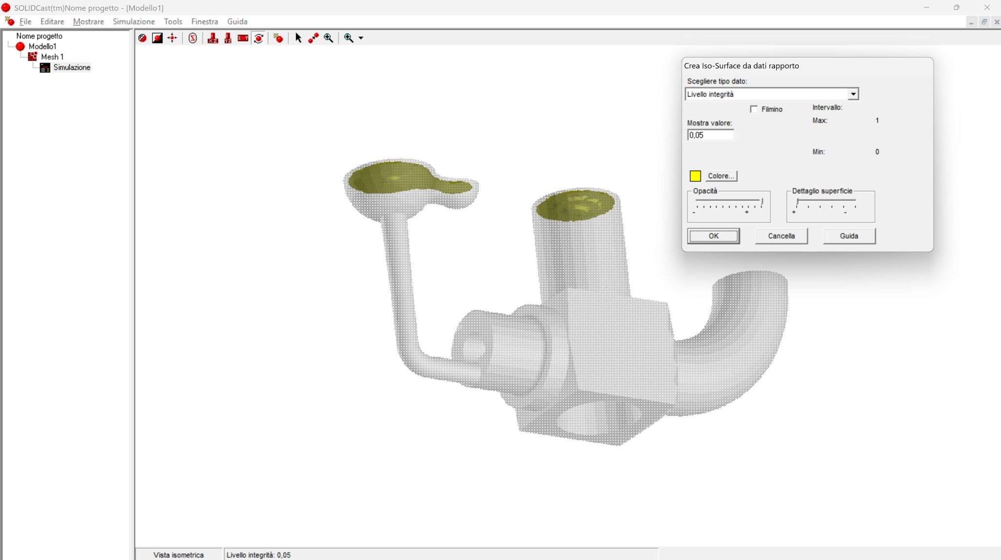

The anomalous shape of the low height shrinkage cone is probably due to the small dimensions of the part compared to the thickness of the shell, whereby heat exchange with the outside is disproportionate.

The program does not allow a graphical representation of areas with porosity above the pre-set probability threshold.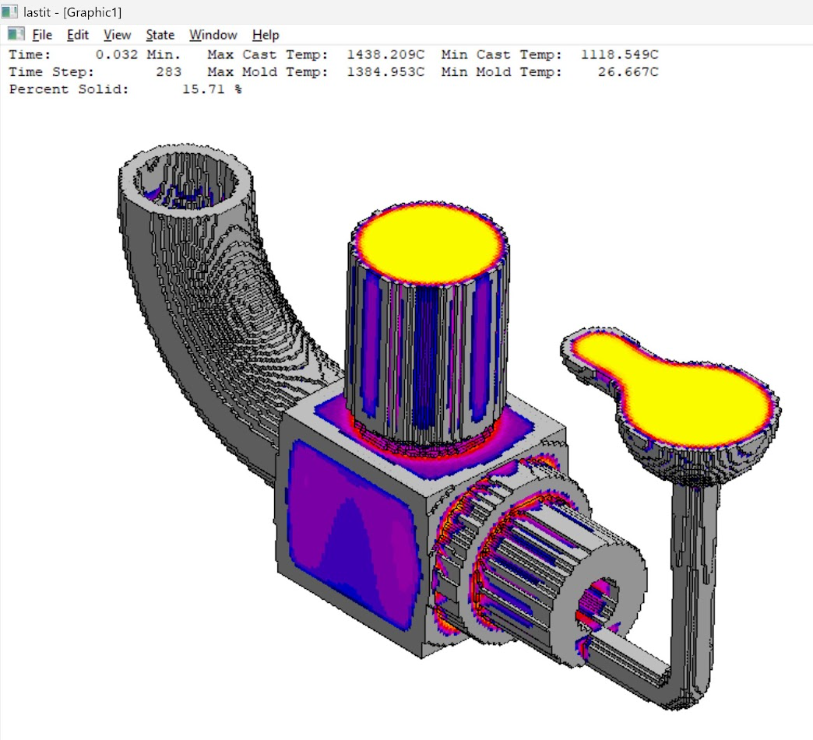

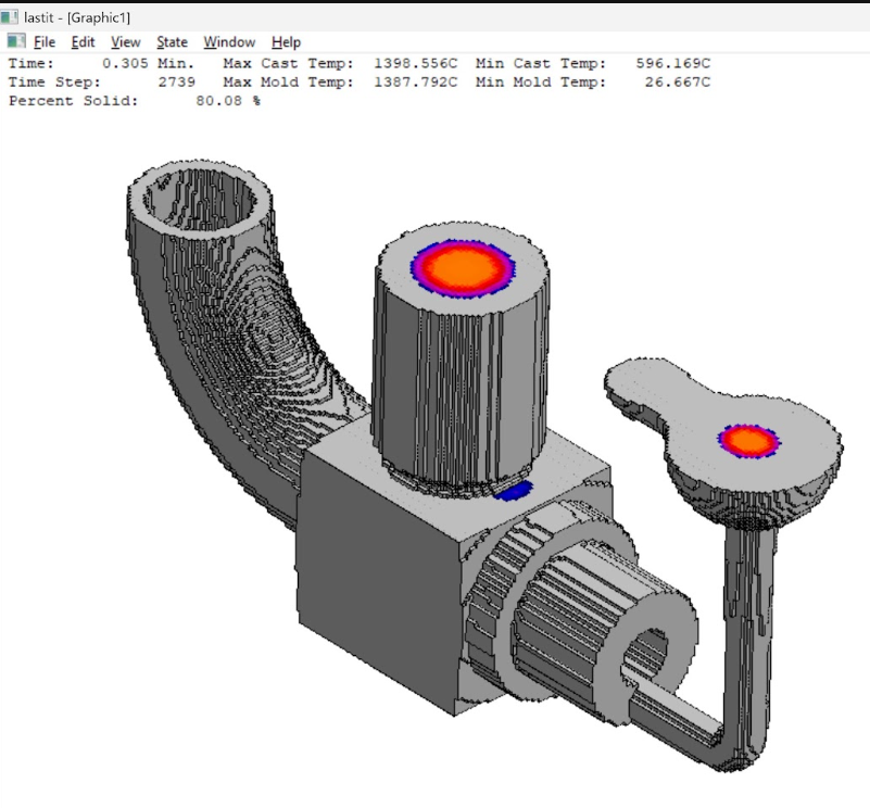
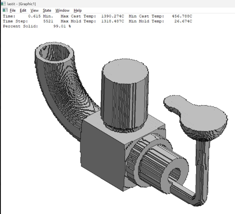
The time required for 80 percent solidification is 0.305 minutes, or 18.3 seconds, compared to the 2 seconds estimated by Chvorinov. This is likely due to the thickness of the shells, which limit heat transfer.

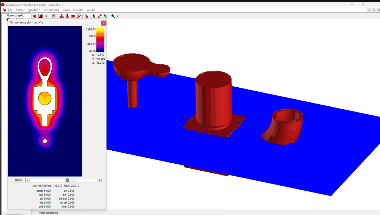
It can be observed that the core remains very hot, so it dissipates little heat and thus creates a hot spot beneath the sprue.

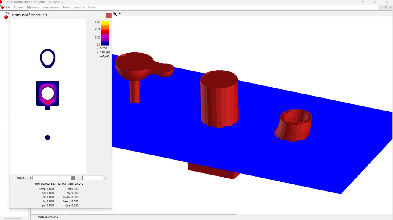
Additional coolers could be considered to accelerate the solidification of the body beneath the sprue.

To conclude, the arrangement and sizing of the feeder, neck, and gating system allow good filling and good solidification, no defects are detected, and therefore this phase can be considered complete.

Process times

We now move on to calculating the "operation times". The term operation means a (simple or composite) operation that is part of the production chain of the casting process, which starts from loading the furnaces and ends with the removal of the feeder and gating system. "Operation time" means the time that a single operation adds to the production time, imagining producing a single piece. From these values we can then calculate:

the total production time of one piece;
the production rate.

Note that the second value is not linked to the first; in fact, since operations occur in parallel, the rate is derived from the time of the operation that constitutes the "bottleneck". Finally, calculating times is fundamental to calculating process costs.

Below are the main operations to take into consideration:

Furnace loading: estimated time of 30 min.
Steel melting: assumed time of 2 h.
Shell forming a: it is assumed that forming phases in general take 5 min.
Shell forming b: 5 min.
Core forming: 5 min.
Mold assembly and placement in container: estimated time of 10 min.
Pouring: 3 minutes estimated for preparation, to which the actual pouring time, provided by software, must be added, but which is negligible compared to preparation.
Cooling and demolding: simulation software calculates roughly 2 s to reach solidification.
Feeder and sprue removal and deflashing: between transport to the designated area, removal/cleaning operations, and storage, 10 min are estimated.

So, assuming we have to produce only one piece and have only one molding machine available, total production time corresponds to about 188 min, i.e., 3 h 8 min.

Since furnaces have high capacity, each time the first two phases are carried out, molten steel is sufficient for many pieces; thus it may be useful to also consider total time excluding the first two phases, which is roughly 38 min.

However, the most significant parameter is the calculation of the effective production rate.

To do this, the bottleneck must be identified.

Phases 1 and 2, for reasons stated in the previous paragraph, can be neglected. Assuming we have a single molding machine, phases 3, 4, and 5 must be performed in sequence and take a total of 15 min. Operations 6, 7, 8, and 9 can be performed in parallel without significant cost increases. Therefore, production time is 15 min.

At this point, the minimum production rate necessary to meet client requests must be calculated.

500 pieces per month must be produced. Assume the foundry is open every day except Sunday, for 12 hours a day. Since there are about 4 Sundays in a month, the production rate is as follows:

minimum production rate = number of pieces per month / 1 working month = 500~pcs/(31-4)working~days= =500 pcs/2712~h=1.5 pcs/h

Breaks and downtimes, which depend on the specific working context, have not been considered.

Since molding time does not exceed the time imposed by the minimum production rate, it is not necessary to parallelize operations and thus a single operator can be dedicated to perform the entire process. Therefore, the production rate can easily be increased by dedicating more personnel to the activity without needing to invest in machinery or equipment.

Process costs

We want to calculate process cost for each piece produced. First of all, main costs must be listed. These include material cost, equipment cost, energy cost, and labor cost. Assuming this is a not-too-small foundry, already existing, and producing other parts besides the commissioned one, and assuming machinery doesn't break down for years, facility maintenance costs are not considered. Machine purchase costs will be amortized.

Material cost

Main materials used are the following:

1. Pre-coated sand: price is about 0.75 €/kg. Considering silica sand density is about 2.6 mg/mm3, sand price corresponds to about 1.9510-6€/mm3. The envelope volume of the two pattern plates is 2(3055100)mm3=3.3105mm3. Therefore, the pre-coated sand cost for each piece is 0.64 €/pc.

2. Stainless steel ASTM AISI 316: the average price of AISI 316 steel scrap is 2000€/ton. To calculate the mass used to produce a piece, feeder and sprue mass must be excluded, as once removed they are recycled. Casting shrinkage should also be considered, but it's not very significant percentage-wise for an approximation; besides, part of the feeder neck stays on the piece.

Therefore, we get: C2= * V *price =8.0 kg/dm39841.0272~mm32000€/ton=0.15€/pc.

3. Optional: Calcium stearate, to be sprinkled on pattern plates to facilitate demolding.

4. Optional: Exothermic sand to cover the open surface of the feeder, to keep it liquid.

Regarding the last two points, since they are powders for surface coating, amount used is assumed tiny and thus cost is neglected.

Equipment cost

Equipment used includes the following:

5. Basic foundry equipment (furnaces, crucibles, workers' tools, etc.), which however are used by all processes and thus amortized according to the following calculation:

annual working hours = monthly working hours * 11 (considering a month of closure) = 1600 h=9.6104min

purchase cost =20k€

amortization time =20 years

annual amortization cost Ca: 20,000/20years=1,000€/year

Cost per minute = 1,000€/year/96,000min/year=0.010417€/min

Amortization quota per piece =0.42€/pc

6. Process equipment, specific to molding type used (machinery to make shells, inserts, and cores, containers and filler materials where mold is inserted for pouring, slag filters, etc.).

Since investment cost is decidedly lower than furnace cost estimated in previous point, calculation is omitted.

7. Equipment to produce the part under examination, like pattern plates. To purchase cost, maintenance cost should be added. Regarding pattern plates and core boxes cost we estimate:

15 mm55 mm100 mm8 kg/dm32€/kg (construction steel (C40) cost) = 1.32 € for each plate or core box half. In total 2 pattern plates and 2 core box halves are needed. They are assumed not to wear out for the entire production which is assumed to last 5 years, i.e. for a total production volume of 5 by 11 months by 500 pcs = 27500 pieces.

Unit cost is: C7=(1.32€+2500€(outsourced CNC machining and purchase cost))4/27500 pcs=0.36€/pc

Energy cost

Energy used, neglecting facility base energy, must:

8. bring steel from room temperature to pouring temperature;

9. heat pre-coated sand to make it polymerize and thus obtain shells, and core;

10. compress air and blow it between core box and cover together with pre-coated sand, if a compressed air system is used.

To calculate point 8 energy, sensible heat and latent heat of fusion should be considered. The first, then, would be an integral of specific heat over dT, calculated from room temperature to pouring temperature. However, this calculation would be too complicated, so specific heat at 20C, equal to 500 J/(kgK), is used. Latent heat of fusion is instead about 2.80105 J/kg.

Finally, the efficiency of furnaces where steel is melted must be considered. Being a typical industrial reality value, eta = 60% is assumed. The volume, moreover, is that of the casting since it's necessary to also heat metal from recycled feeder and gating systems. So:

E =1/60% * 8,0 kg/dm3 ⋅ 16.607 ⋅ 103 mm3 ⋅ (500 J/kgK ⋅ (1813,15 K − 293,15 K) + 2,8 ⋅ 105 J kg) ≃ 0.23 MJ/pz

Assuming used furnaces are electric and considering electric energy price is about 0.23€/kWh, which corresponds to about 0.06€/MJ, the calculation is 0.0147€/pc.

For point 9, silica sand specific heat is about 0.27~kcal/(kgC), corresponding to about 1130~J/(kgK). Although this specific heat is more than double that of steel, since the temperature to reach is around 200C and given the low cost of electric energy, this cost can also be neglected.

Labor cost

Labor cost essentially consists of foundry workers' costs.

Since they are specialized workers, cost for the company is estimated at about 28 €/hour. Cost of workers involved in phases 1 and 2 is neglected, being operations non-specific to the process and not requiring constant presence of a worker. For molding phases, as estimated, one worker is enough. For mold preparation, pouring, and casting demolding, dedicating a single worker, a total time of 30 min was estimated to execute all operations in series except feeder and flash removal. Considering productivity is thus 2~pcs/h, total labor cost for each piece produced is then 28/2=14€/pc=Cm.

Total cost

Total cost is therefore: Ctot = C1 + C2 + C5 + C7 + Cm = (4 + 16 + 56) €/pc = 15.58 €/pc

Variant to be welded

For educational purposes, a part variant to be welded is planned in addition to the one to be screwed on, to be studied. Being a family of parts (group technology), to avoid costs of an additional pattern plate as suggested by Kalpakjian textbook, an insert is planned to create in the mold a cavity that will generate the threaded part, which is totally absent in the part to be welded.

Component drawing is shown in the welding chapter.

Welding

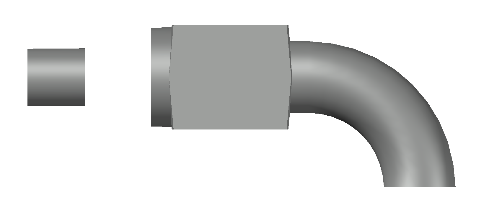
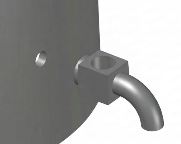
As indicated for the welded part variant, an economic version of barrels with a welded tap is planned as an alternative to the demountable version, sold as a separate product, which can instead be screwed/unscrewed to other types of barrels/receptacles/containers.

Choice of process

To perform the welding as in the figure, we choose an autogenous fusion welding with coated electrode electric arc. This welding indeed has low costs thanks to cheap welding machines and low skills required of welders. The 2 mm barrel thickness presents no risk of burn-through.

Welding position

Furthermore, it is applicable in different positions thus allowing execution flexibility with the part fixed or with any orientation (horizontal or frontal).

Metal preparation

Given the small dimensions of the piece and the circular ring geometry, edge preparation (beveling) is not necessary, always with a view to high economic efficiency.

Choice of electric arc welding machine

As an electrode welding machine, we use the Telwin Technology 186~HD/XT in direct current (DC) with rutile, acid, and basic electrodes (they guarantee excellent arc stability and easy slag removal on thin thicknesses like 2 mm).

Data sheet

GENERATOR CHARACTERISTICS

Power supply 230V 1ph 50/60Hz

Maximum no-load voltage 60V

Quick connectors Ø 13mm

Protection degree IP23

Connectability to power generators YES, tolerance +/- 15%

MMA WELDING

Current adjustment 5 - 160A

Duty cycle 160A 35%

Absorbed power 60% 3.3 kW

Rutile, inox electrodes Ø max 4.0 mm

Basic, cast iron electrodes Ø max 3.2 mm

LOGISTICAL DATA

Item dimensions 375 x 220 x 500 mm

Item weight 10.1 kg

Cost €436.00

Machine cost

Parts and tools participating in the process are:

electrode holder gun
ground clamp
electrodes
metal to be welded

Considering a purchase cost of 436 € also inclusive of necessary accessories and equipment, and assuming a 5-year amortization and an utilization equal to half a shift (4 hours/day) on the 6 operational days per week of the company, for 44 working weeks, i.e., 4*6*44*60=1056 h=63360 minutes meaning 316800 in 5 years, we obtain a cost of 0.00138€/min (0.0826€/h).

Choice of coated electrodes

Considering small part dimensions and 2 mm sheet thickness, among the smallest rutile coated electrodes specifically for austenitic stainless steels type AISI 316L are chosen, with 2.0 mm diameter and 300 mm length. Below is the technical data sheet.

Modello DAIKO G-TECH 316LR

Fornitore Laboratorio Saldatura

Materiale Metallo Base Acciaio Inossidabile AISI 316 / AISI 316L

Classificazione AWS A5.4: E316L-16

Tipologia Rivestimento Rutile-basic

Diametro Elettrodo 2 mm

Lunghezza 300 mm

Corrente Operativa Consigliata 40 - 60 A (Corrente Continua DC+)

Confezione industriale da 145 pezzi

Prezzo Confezione 57.00 €

Costo Unitario per Elettrodo 0.393 €/elettrodo (57 € per 145 pz)

Consumable material cost

Electrode consumption is equal to the volume of material deposited to make the bead. We assume a bead height equal to 1/3 of the ring 4 mm long, equivalent to 1.33 mm, equivalent to a roughly triangular section of 0.89 mm2, corresponding to a volume of 53.08 mm3 considering bead perimeter of 59.71 mm.

Volume of an electrode with indicated characteristics of 2 mm diameter and 300 mm length and considering a 65% real yield is 42.4*0.65=612.61 mm3.

So electrode consumption equals 8.66% and thus a cost of 0.034 €/pc.

Welding time

We assume a speed of 3 mm/s so for a 59.71 mm length it will take 20 s.

Labor cost

Operator cost = 25€/h.

The gross hourly company cost of the indicated welder is lower than that of the shell molding operator (28€/h) given the lower degree of specialization required. Considering the 20 s time employed for each weld, the welder cost will be 0.1389 €/pc, increased by about 10% to account for costs of setting up the welding station for each lot.

Welding energy cost

Energy needed equals the volume of an entire bead times the cost expressed in E/mm3 to melt inox steel. Since electrode material must be compatible with part material, we consider energy costs to bring it to fusion, already determined in the casting section, corresponding to 0.0007 MJ for the weld bead, corresponding therefore to 0.00005 €/weld (with a 70% efficiency).

Welding machine parameters

Given material fusion energy equal to 0.01387 kJ/mm3, considering a 20 s/piece time, machine power will have to be 1.25 kW (accounting for thermal dispersions and arc efficiency). Setting a voltage of 25 V, not too high to avoid burning through the barrel sheet, we derive a current of 50 A. Current will be alternating to reduce magnetic blow and keep a balance between deposition and penetration.

Total welding cost [€/pc]

Machine cost = Welding machine amortization cost * welding time * 110% = 0.00138 €/min * 20 / 60 min * 110\% = 0.00051

Material cost = Electrodes cost / number of pieces = 0.393 €/electrode * 8.66% electrode = 0.03403

Labor cost = Operator cost * welding time (+10%) = 0.1389 €/pc * 110% = 0.15279

Energy cost = Energy cost / mm3 * Bead volume = 0.00005 €/weld

Total = 0.187

Plastic Deformation

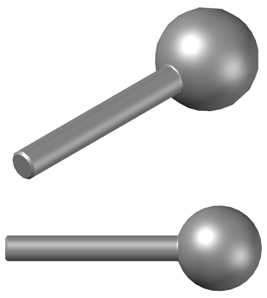
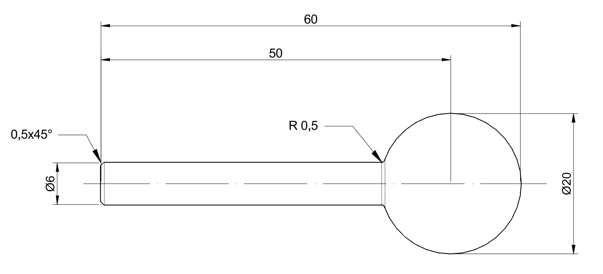
Part choice

As the part to be made by plastic deformation we have chosen the knob. This is because it allows obtaining it as a single piece and avoids the waste of material that would occur with chip removal, given the considerable difference between the diameter of the knob and that of the rod. Furthermore, being a dynamic element, often subjected to bending and shear (and therefore susceptible to fatigue phenomena), the plastic deformation process improves its mechanical characteristics thanks to phenomena such as strain hardening and grain flow (i.e. a more homogeneous rearrangement of the grains).

However, the considered part requires geometric adaptations in order to be actually made by stamping:

The rod has a length-to-diameter ratio that exceeds the recommended values to avoid buckling (L<2.53D)
The ratio between the diameter of the knob and the rod exceeds the recommended limit of 1.8
There are parts not sufficiently chamfered or filleted, technologically impossible.

Therefore, the following modifications are applied to the part:

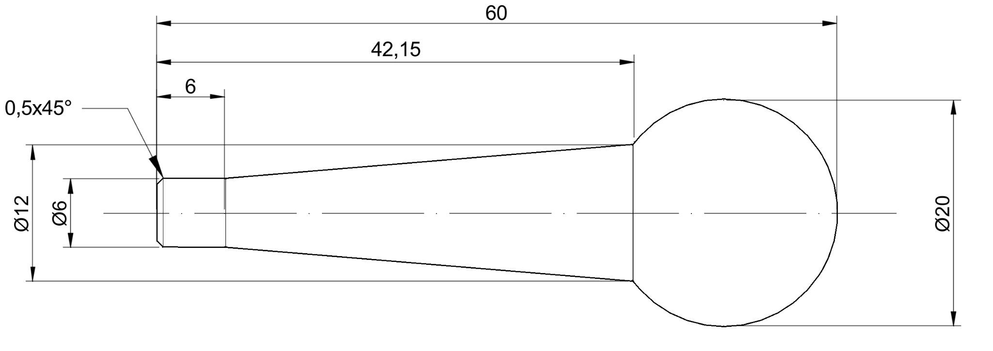
The first 6 mm starting from the end at diameter 6 mm are kept
A gradual increase in diameter up to 12 mm is made when it reaches the knob, which instead remains of unchanged diameter for ergonomic reasons.

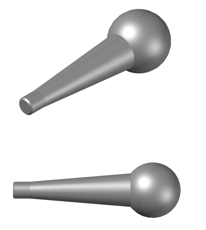
Modified part

Choice of material

For the knob we decided not to keep the same material as the rest of the dispenser (AISI 316 Stainless Steel (EN 1.4401)) because it is too difficult to machine by stamping due to the marked tendency to work-harden. However, given the need to connect the knob to the plug, it is not possible to use high ductility materials like aluminum or brass because galvanic corrosion phenomena would be created. Therefore the choice falls on another Stainless Steel that thanks to the addition of copper becomes much more workable by stamping: AISI 304Cu Stainless Steel (EN 1.4567).

	AISI 304Cu Stainless Steel (EN 1.4567)
Yield strength (Rp0.2)	175 MPa
Tensile strength (Rm)	450-550 MPa
Elongation at break (A)	> 50%
Strength coefficient (K)	1100 MPa
Strain hardening exponent (n)	~0.45

Choice of the starting billet

As a starting blank a cylindrical billet is chosen. To minimize the forces necessary for carrying out the process, an intermediate diameter between the max one of the knob (20 mm) and the min one at the end of the rod (6 mm) is used, for convenience we chose the 12 mm one at the attachment point between rod and knob.

At this point I can calculate the length of the billet starting from the volume of the finished part (V=6613.98~mm3), considering material losses due to flashes negligible: A0=D02/4=3.1436~mm2=113.04~mm2 L0=VA0=6613.96~mm3113.04~mm2=58.51~mm

Calculation of the upsetting ratio

Upsetting ratio

It serves to determine the number of stages required for the press (if greater than 2.5 it is necessary to add a second stage). To calculate it I must first obtain the volumes of the rod and knob: Vrod=Vcylinder+Vtruncated cone Vcylinder=626=169.6~mm3 Vtruncated cone=(42.15-6)12(122+126+62)=2384.5~mm3 therefore Vrod=169.6+2384.5=2384.5~mm3 Vhead=Vtot-Vrod=6613.98-2384.5=4059.9~mm3 I calculate the equivalent length of the head (i.e. how long a cylinder of diameter 12 must be to have the same volume as the head): Lhead=VheadA0=4059.9~mm3113.10~mm2=35.9~mm Obtaining an upsetting ratio equal to: LheadD0=35.9~mm12~mm=2.99>2.5 I must therefore perform the machining with a 2-blow machine

Formulas and calculations

Parameter	Symbol	Formula	Calculations
Total volume of the part	V	Initial data	6613,98mm3
Starting wire diameter	D0	Chosen based on max diameter of truncated cone	12mm
Wire cross-sectional area	A0	D024	1224=113,10mm2
Theoretical cutting length	L0	VA0	6613,98113,1058,48mm
Free length to upset	Lh	VheadA0	4059,9113,1035,9mm
Upsetting ratio	R	LhD0	35,9122,99>2,5 so it requires 2 blows
Projected area spherical head	Aproj	Dsphere24	2024314,16mm2
True logarithmic strain		ln(AprojA0)	314,16113,101,02
Average flow stress (Hollomon's Law)	f	Kn1+n	12001,020,451+0,45834 MPa
Maximum flow stress (Hollomon's Law)	f,max	Kn	12001,020,451210 MPa
Stamping force (Finishing)	F	AprojfCp	314,168342,5=655996 N (around 65 tons)

Choice of process

To make the part I choose the upsetting process (cold stamping), preceded by an extrusion phase (roughing).

Choice of machine and equipment

Main Machinery: Stamping Press

As the main machinery, the 2-Die 2-Blow cold mechanical horizontal Stamping press with slider-crank kinematics was chosen.

This choice was made because the slider-crank kinematics slow down the stroke near the bottom dead center, allowing the material to flow plastically without cracking. The 2-die configuration is mandatory because the upsetting ratio (2.99) exceeds the limit of 2.5 for a single blow, making an intermediate roughing phase necessary.

Parameter choice
Parameter	Value	Reason
Tonnage (Nominal Force)	80 Tons	A 30% security margin was added to the required 60 Tons
Production speed	60 strokes/min (ppm)	Stainless steel generates a lot of heat due to friction and deformation, therefore working at lower speeds compared to common steels allows lubricants to dissipate heat, avoiding galling and premature tool wear.
Slider stroke (Stroke)	125 mm	The finished part is 60 mm long. The slider must retract at least twice this size to allow grabbing the ejected part without collisions with the moving punches.
Extraction force (Kick-out force)	10 Tons	The extrusion of the shank, with its high upsetting ratio, generates enormous radial pressure on the die. This causes the part to stick to the walls, therefore a substantial extraction force is needed to be able to eject the part.
Extraction stroke	65 mm	The shank penetrates deeply into the die, therefore the ejector pin must have a stroke greater than the total length of the part (60 mm) to push it out completely.
Cutting capacity (Cut-off)	12 mm	The machine must be able to shear the starting wire which is 12 mm in diameter.

Tooling components

The tooling setup is proportioned to very severe cyclic loads and typical abrasiveness of AISI 304Cu.

Components	Characteristics	Reasons
Insert Material (Dies and Punches)	Tungsten Carbide (Widia / Hard Metal)	Hard metal guarantees the necessary wear resistance, maintenance of surface polish and very high compressive strength.
Cutting knife and bushing	Must have tight tolerances.	A slanted or burred cut would cause the wire to skid on the first blow.
1st Punch (Rougher)	Features a "barrel" cavity.	The specific cavity serves to rough out the wire (i.e. to partially flatten it) increasing its diameter and reducing its length, to bypass the risk of instability and prepare the perfect volume for the spherical head.
Forming (and upsetting) die	Tapered internal profile (from 12 to 6 mm).	Forces the metal to extrude forward forming the conical shank, and acts as an anvil for the blows of the upper punches.
2nd Punch (Finishing)	Features a perfect mirror polished hemispherical cavity (ø20 mm).	Closes the roughed volume from the first punch in a closed die: the final spherical geometry is generated.
Ejector pin (Extractor)	Shaped to hit the bottom of the shank (ø6 mm). Includes the negative of the 0.545 chamfer.

Auxiliary Systems and Lubrication

Given the natural tendency of stainless steel to cold galling, machining must be performed with careful lubrication:

Wire preparation: Oxalation

Reason: The virgin ø12 mm wire in AISI 304Cu cannot be stamped without receiving a pre-drawing chemical treatment: an oxalate coating combined with calcium/sodium stearates, which acts as a sponge to retain oil during extrusion.

Stamping oil: Neat EP (Extreme Pressure) oils

Reason: Very high viscosity oils with sulfur, chlorine or phosphorus additives are used. Additives that activate at high local temperatures generated by stamping, creating a solid chemical barrier between die and part.

Machining cycle

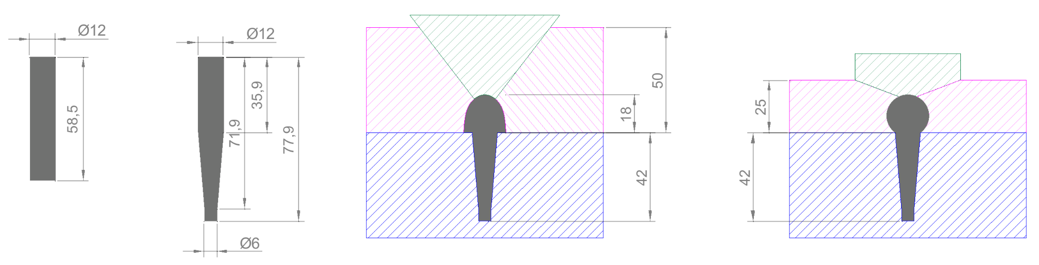
Roughing (First die)

reduction of the shank from 12 to 6 mm diameter with an extrusion process
preliminary upsetting of the head: the 35.9 mm part is preliminarily formed into a barrel shape to accumulate material without generating buckling.

Finishing (Second die)

creation of a spherical knob with a closed die.

Time calculation

Considering a batch of 500 pieces/month, production times are calculated by conservatively setting the speed for AISI 304Cu at 60~strokes/minute.

Phase	Description	Time (min)	Time (h)
Setup	Changing dies, punches, cutting and centering. (Complex manual operation).	180.0	3.00
Production Cycle	Continuous stamping at 60 ppm (500~pcs/60).	8.3	0.14
Total Batch Time	Physical occupation of machine and operator	188.3	3.13

Cost calculation

For the calculation, we assume a standard industrial setup where the machine is inserted in a production department (amortization distributed over 1600 hours/year on a single shift) and the batch cost is absorbed based on occupied machine time. Otherwise, the initial investment would not be justifiable for such a small batch.

Machinery Selection and Investment (New)

To machine a 12 mm diameter wire with a nominal force of 100 Tons, reference is made to a top-of-the-range European 2-die stamping press (e.g. SACMA SP 270 or Carlo Salvi CS 513).

Machinery: Cold press including everything.
Investment value: € 450,000.
Amortization (10 years): € 45,000 / year.
Base hourly machine cost (amortization quota only): € 45,000 / 1600 hours 28.12~€/hour. Adding energy costs, lubricants and ordinary maintenance, a complete machine cost of 45.00 €/hour is estimated.

Cost Analysis (Batch of 500 pcs)

The blank weight was calculated from the initial volume (V=6614~mm3) which with the density of AISI 304 (7.9~g/cm3) is equivalent to about 0.052~kg/piece.

Cost Item	Calculation Parameters	Total Batch Cost	Cost per Piece
Material (AISI 304Cu)	Net requirement: 26 kg. Setup waste (5%): 27.5 kg total. Price: 5.50 €/kg. (Source: LME Nickel index + inox alloy surcharge)	€ 151.25	€ 0.302
Machine Quota	3.30 hours x 45.00 €/hour (amortization + consumables).	€ 148.50	€ 0.297
Direct Labor	3.30~hours35.00~€/hour (toolmaker/specialized operator).	€ 115.50	€ 0.231
Tooling Quota	New Widia die set: €5,000. Estimated useful life: 100,000 pieces (more than total production in 10 years). Incidence: 0.05 €/pc.	€ 25.00	€ 0.050
TOTAL	Industrial cost	€ 440.25

Additive Manufacturing (3D Printing) & DfAM

Characteristics of the knob

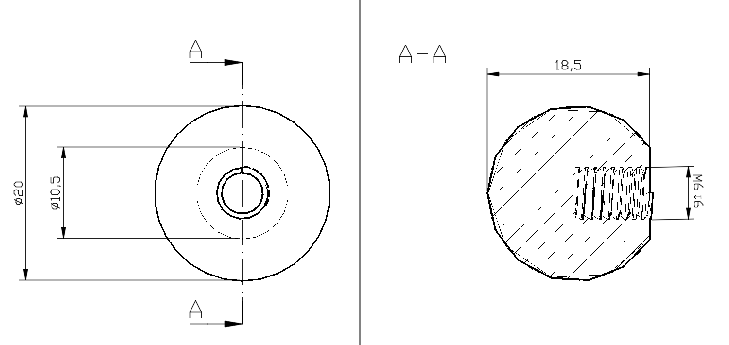
The grip knob for opening/closing the tap has a hole for hot insertion of a threaded metal insert, or directly of the metal rod, to allow stable and durable coupling. Thermoplastic polymer characteristics common to all FDM materials are exploited. The original component has a threaded hole for coupling, as shown in the figure.

Even if in principle a thread would be printable according to the machine supplier, this solution is avoided as it presents numerous practical problems and does not guarantee durability over time.

Choice of FDM process

As anticipated, among 3D printing techniques for polymers, we opt for FDM (vs. VAT) for non-stringent dimensional requirements and better cost-effectiveness and technology diffusion.

Choice of knob material

Polymer must be printable for educational requirements.

It must have high mechanical properties being continuously stressed, including resistance to humid environments and heat, therefore common PLA is discarded, which is rigid but brittle under continuous stress and suffers from humidity and heat.

PETG has excellent mechanical resistance, resists water/humidity better, has slight elasticity that aids coupling, and prints easily on the Prusa without warping.

Coupling temperature will be between 210C and 230C, range indicated for printing. At glass transition temperature of 80C material will not allow easy metal insertion.

Geometric tolerances of the knob

For modifying the hole on the knob, an interference fit for plastic-metal couplings between 0.2 mm and 0.3 mm on the internal diameter of the knob thread is planned. Hole diameter must be greater than 6 mm (current thread diameter).

A small chamfer (451~mm lead-in) is also planned at the entrance of the knob hole to facilitate insertion.

Choice of FDM machine

We opt for Prusa One+, established brand, mid-high end model suitable for industrial production. Data sheet:

Print volume 250 × 220 × 270 mm

Filament diameter 1.75 mm

Layer height 0.05-0.30 mm

Printer dimensions 22.5 kg, 415 × 444 × 555 mm; 16.3 × 17.5 × 21.8 in (X×Y×Z)

Mainboard Custom 32-bit xBuddy electronics with STM32

Stepper drivers Trinamic 2130

Stepper motors Precise 0.9° stepper motors in X and Y (prevent VFAs)

Extruder Nextruder, direct drive, E3D V6 compatible (with adapter)

Extruder electronics Custom expansion board to connect fans, thermistors and other components

Filament path Aluminum heatsink, all-metal hotend

Drive system Nextruder planetary gear system, 10:1 gear ratio reducer

Cooling fan High performance turbine, 360° cooling system

Nozzle Prusa CHT High Flow brass nozzle - 0.4 mm

Max nozzle temperature 290 °C / 554 °F

Max heatbed temperature 120 °C / 248 °F

Max chamber temperature 55 °C / 131 °F

LCD screen 3.5" graphic screen with 65k colors

Touch controls Yes

Firmware update interface USB stick, Prusa Connect, Prusa Mobile app

Prusa Connect support Yes

Quick-Swap nozzle system Yes

Internal camera Optional solution inside chamber

Multi-Material support Yes, MMU3 (5 filaments) and INDX (up to 8 filaments)

HEPA filtration Optional add-on

Connectivity Ethernet, Wi-Fi (NFC receiver, optional Wi-Fi module)

Filament sensor Yes (2 sensors)

Load Cell sensor Yes

Print surface Magnetic heatbed with flexible PEI steel plates

First layer calibration Fully automatic (load cell sensor)

Input shaper Yes

Supported materials PLA, PETG, Flex, PVA, PC, PP, CPE, PVB (Advanced: ABS, ASA, HIPS, PA)

Power supply 240W with Hardware Power Panic

Power consumption PLA: 90W / ABS: 110W

FDM machine depreciation cost

Considering a purchase cost of 1350 € also inclusive of necessary accessories and equipment, and assuming a 5-year amortization and an utilization equal to half a shift (4 hours/day) on the 6 operational days per week of the company, for 44 working weeks, i.e., 4* 6*44*60=1056 h=63360 minutes meaning 316800 in 5 years, we obtain a cost of 0.00426 €/min (0.2557 €/h).

Printing parameters

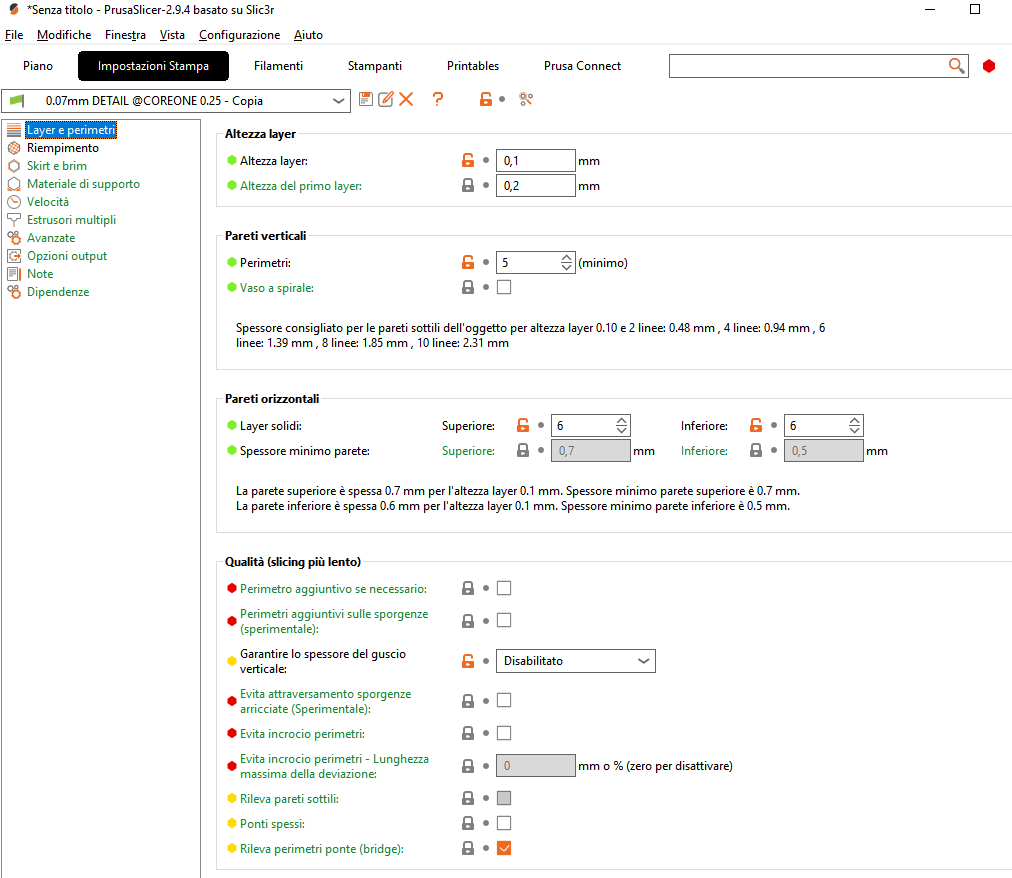
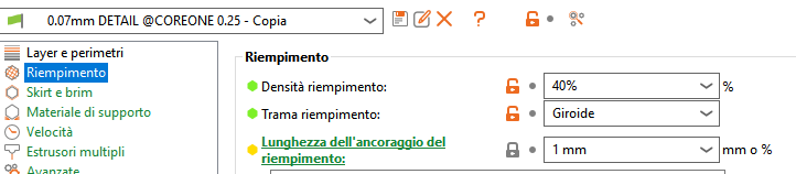
Choosing Advanced/Expert mode, the following parameters are set to achieve the desired mechanical resistance:

Orientation on the bed: hole is facing perpendicular to the print bed, ensuring circularity and geometric tolerance of the hole.
Layer height (Layer Height) low: equal to 0.10 mm (Quality) to favor better aesthetic quality of the external spherical surface, mitigating the stair-stepping effect.
Infill: 40% density with Gyroid pattern, for higher torsional resistance.
Perimeters (Shell): 5 vertical perimeters of solid, full plastic around the hole and external surface, to prevent the metal rod and user from breaking through the internal structure.

Part orientation

Hole with vertical axis for reasons indicated above regarding surface quality.

Oriented downwards to have a larger adhesion area to the bed, corresponding to the circle surface. This would also have the advantage of not having to rework the opposite spherical surface.

Conversely, support material inside the hole will be needed to support the bottom of the hole. A hole bottom inclined at 45 degrees would not require support structures, but would further weaken the knob internally. Support structures are also planned for a good part of the spherical surface surrounding the hole, especially to improve bed adhesion and avoid known phenomena of the part detaching from the bed, dragged by the print head.

Printing time

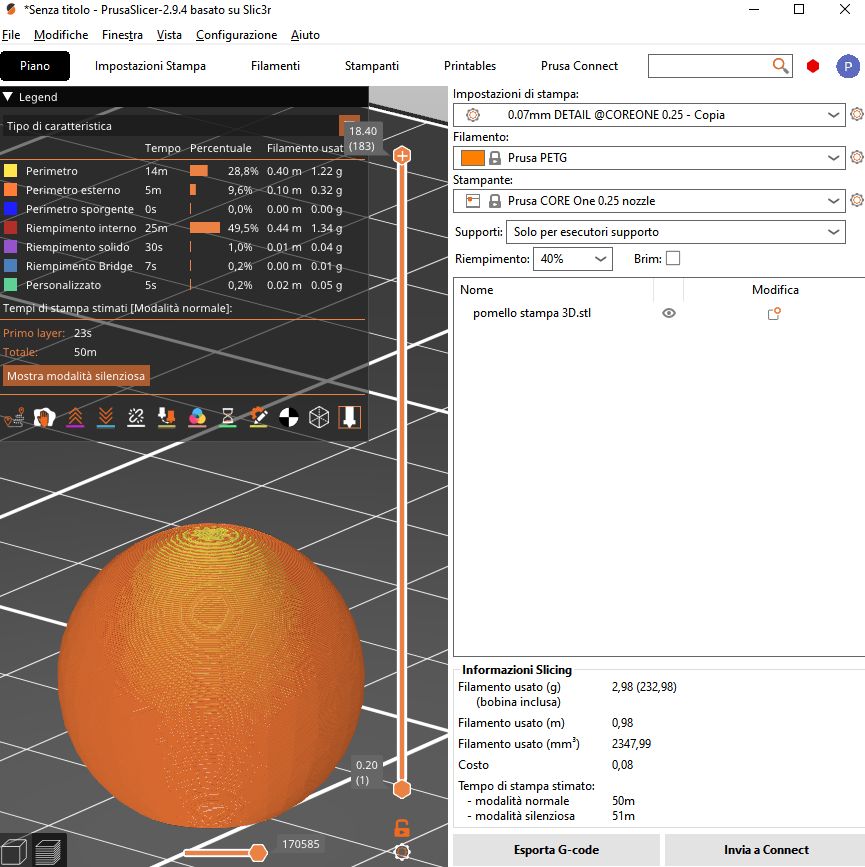
Print time resulting from simulation as per figure is equal to 50 minutes.

Material cost

As resulting from print simulation, the amount of material used for each piece is equal to 2.98 g meaning 0.051 €.

Knob cost

Machine cost = 0.00426€/min50~min=0.213€

Material cost = 0.051€

Total cost = 0.264€

Machining (chip removal)

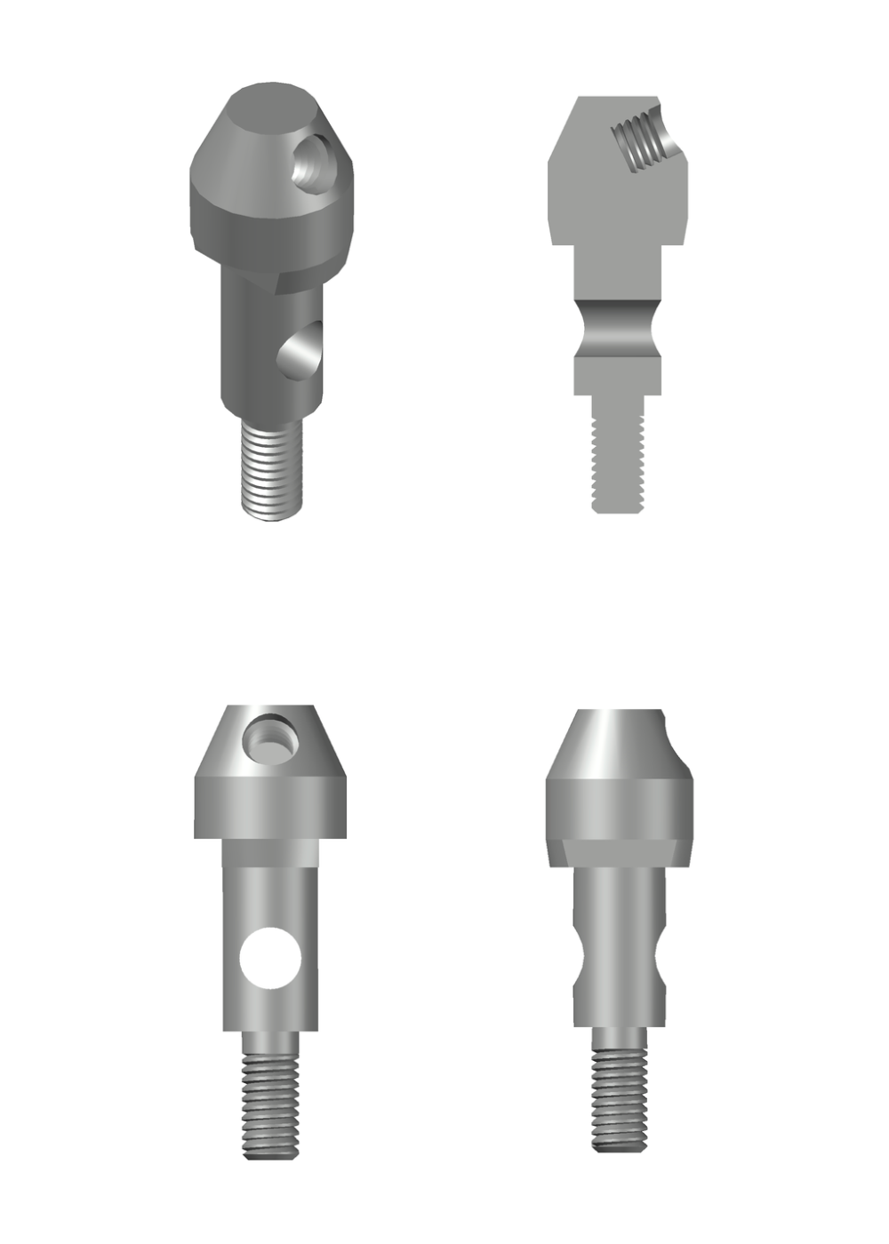
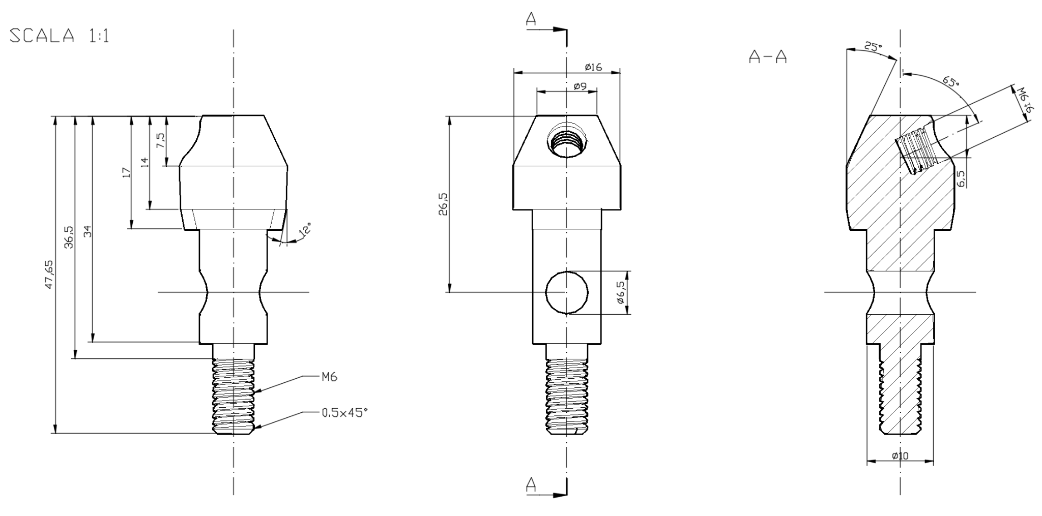
Choice of part

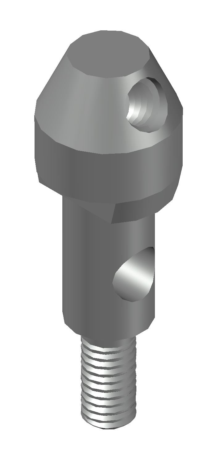
Chip removal machining was chosen as the production process for the cylindrical plug because it is a kinematic part that requires tight tolerances and excellent surface quality. Furthermore, it has complex shapes that are not suitable for plastic deformation manufacturing.

Choice of material and semi-finished product

To make the cylindrical plug, it was decided to use AISI 316 Stainless Steel (EN 1.4401) for its excellent anti-corrosion qualities, given by the presence of 2-3% molybdenum, necessary to guarantee adequate durability in contact with wine, a highly corrosive liquid (acidity and presence of sulfites). However, AISI 316 presents some technological disadvantages: it has low thermal conductivity (it overheats more easily) and a strong tendency to be work-hardened and for chips to adhere. This entails the need for some technological expedients that will be analyzed further on in the report.

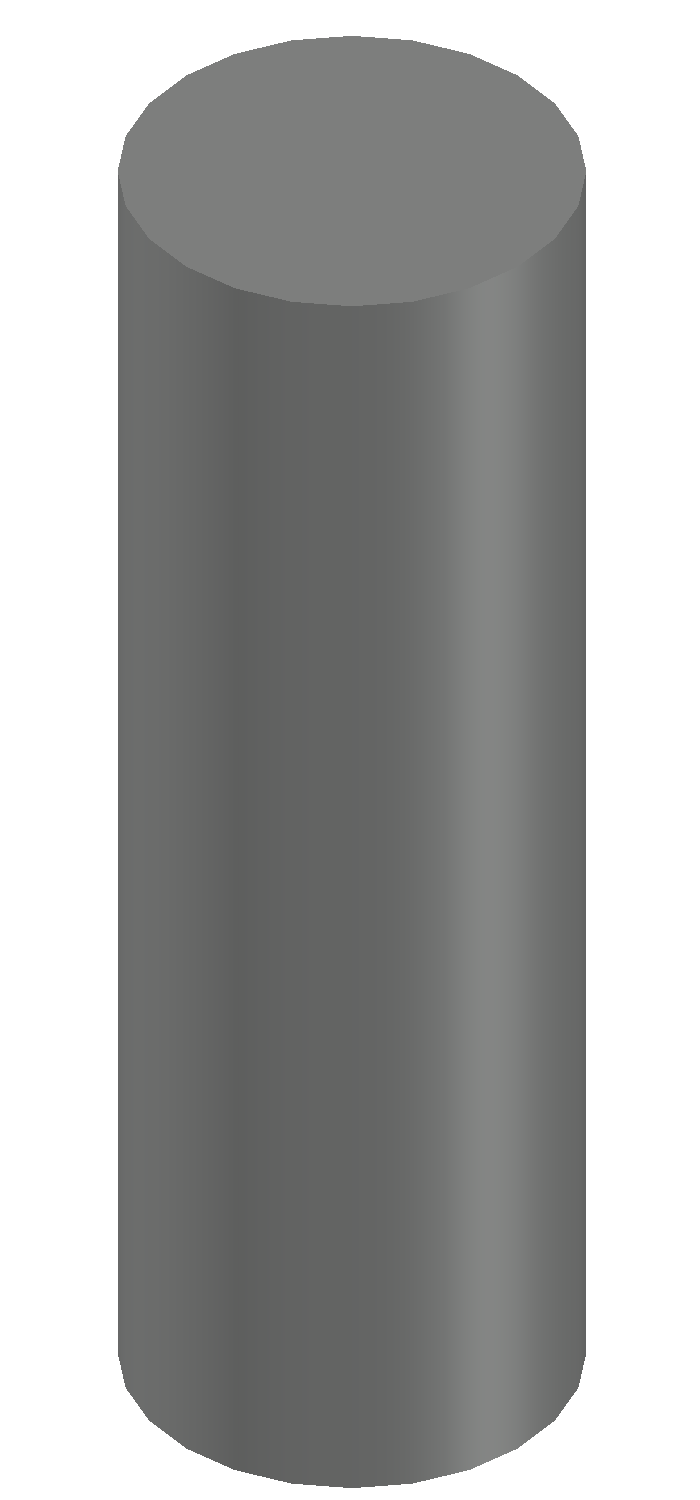
The production cycle starts from a cylindrical bar of the aforementioned INOX steel, made by extrusion and subsequent cold drawing. This semi-finished product, given the part's overall dimensions (16 mm diameter and 47.65 mm length), must have at least an 18 mm diameter (+1 mm machining allowance) and 52 mm length to allow facing (+1 mm machining allowance) and parting off (+3 mm) of the part from the initial bar.

Definition of phases

N°	Machining	Tolerance	Roughness
1 - head	Turning	0.1 mm (ISO 2768-m)	1.6 m
2 - cylindrical body	Turning	h7	0.8 m
3 - thread	Turning	6g	3.2 m
4 - wing housing	Milling	0.1 mm (ISO 2768-m)	1.6 m
5 - hole	Drilling	0.1 mm (ISO 2768-m)	3.2 m
6 - threaded hole	Drilling	6H	3.2 m

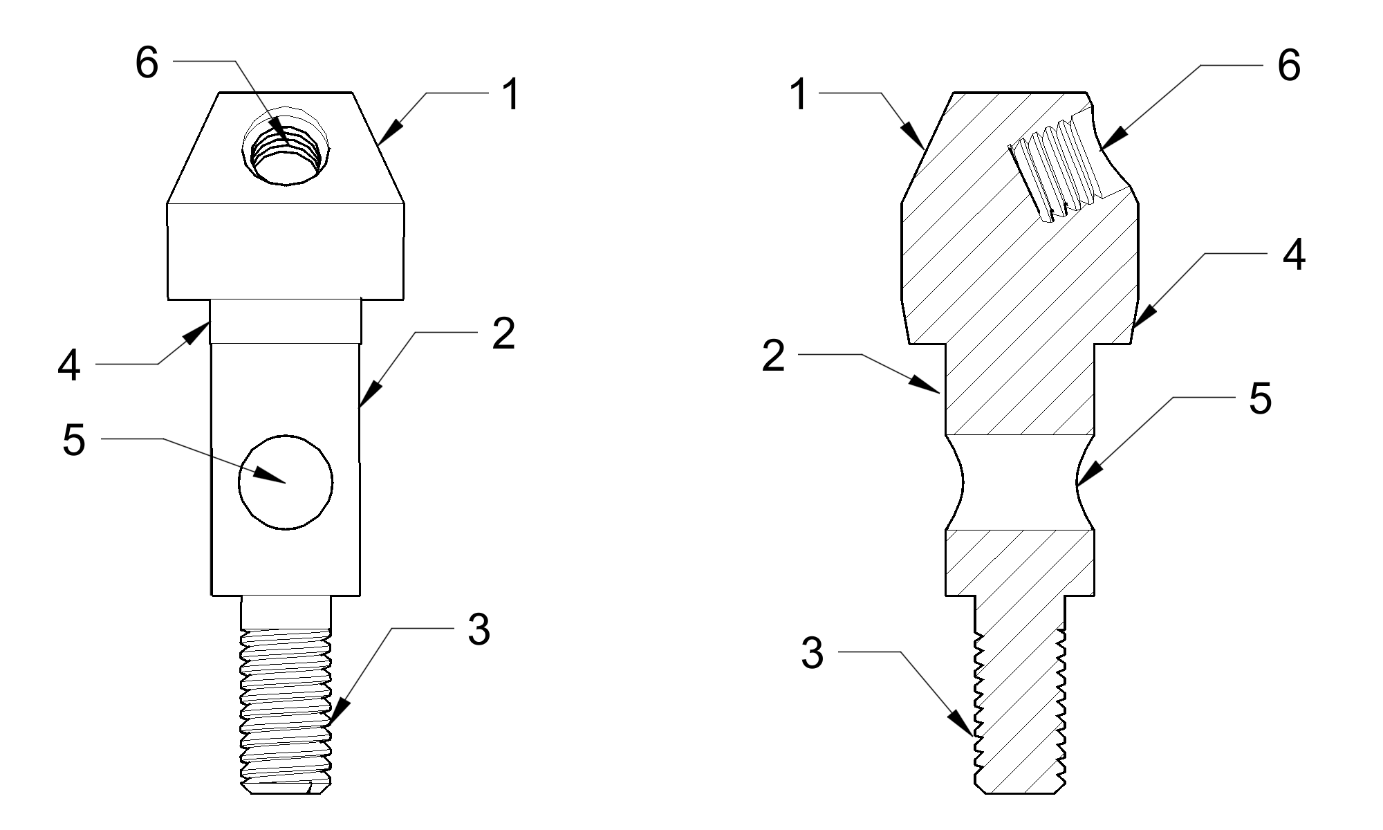
Grouping of phases

Grouping machining operations for chip removal reduces production times and costs. To be effective, it must respect precedents:

Technological: facing and roughing of the external diameter represents the first operation of the cycle, since it allows obtaining the reference surface. It is followed by finish turning and threading, performed on the definitive diameter to ensure the correct profile and respect of tolerances. Once this is done, parting off is performed and, finally, milling, drilling, and tapping are carried out.
Geometric: turning the external diameter must precede the external threading, since this requires a perfectly cylindrical surface to meet dimensional specifications. Subsequently, milling occurs and, finally, drilling is performed, using the part's axis as a geometric reference, so as to obtain correct positioning and sizing.
Economic: executing turning first allows verifying semi-finished product conformity, since it removes the bulk of the material. Then, given the complex nature of this machining, it is good practice to proceed with thread creation, so as to be able to discard defective parts before subsequent operations. The same goes for holes: first the threaded one is performed to avoid risking damage to the part in the final phases of the process.

In the analyzed case:

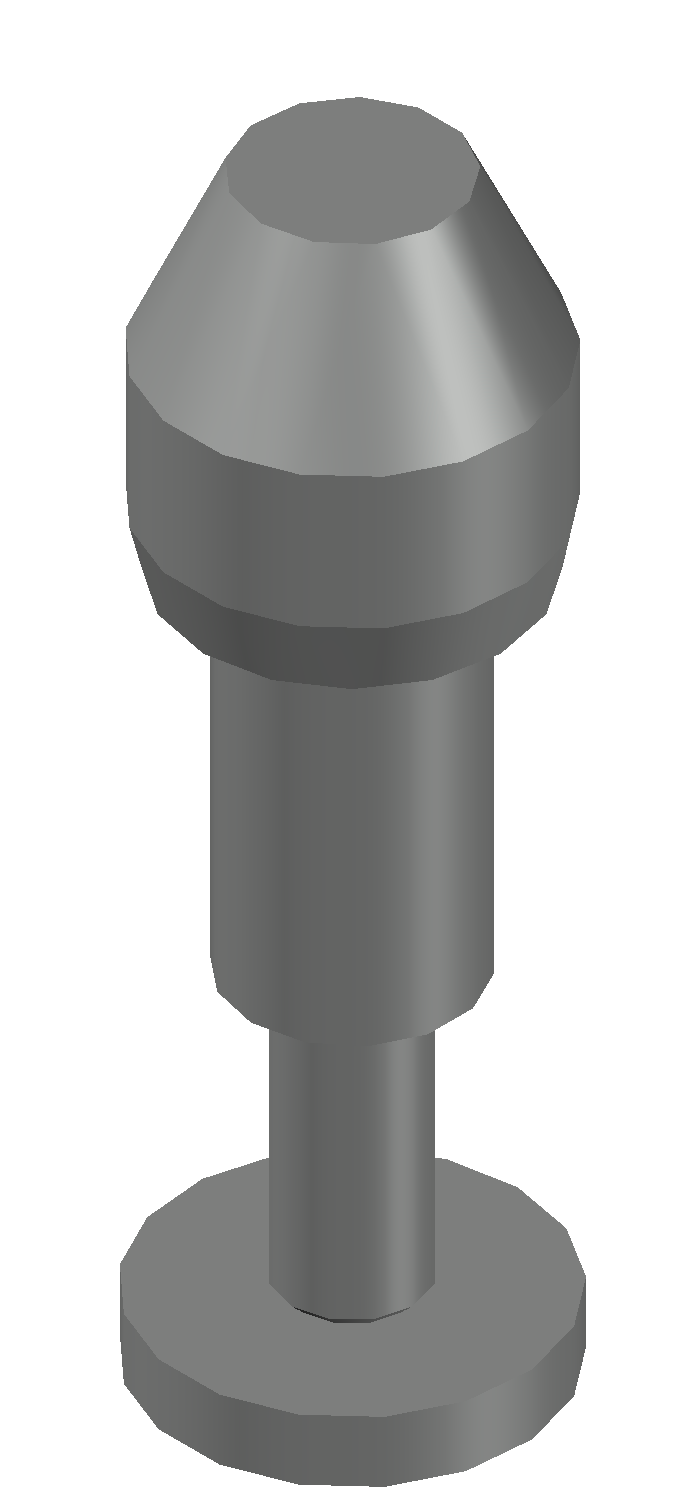
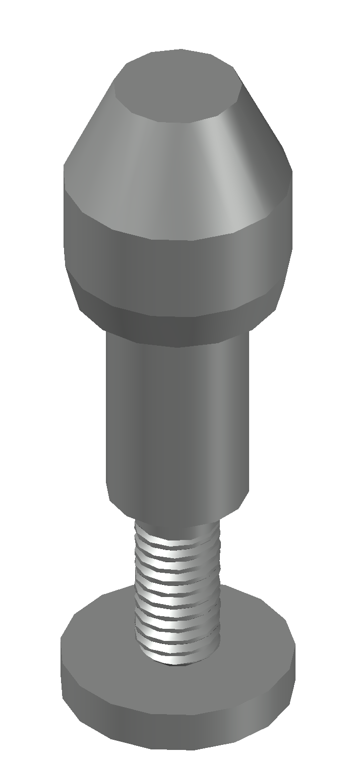
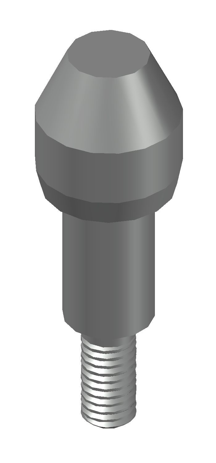
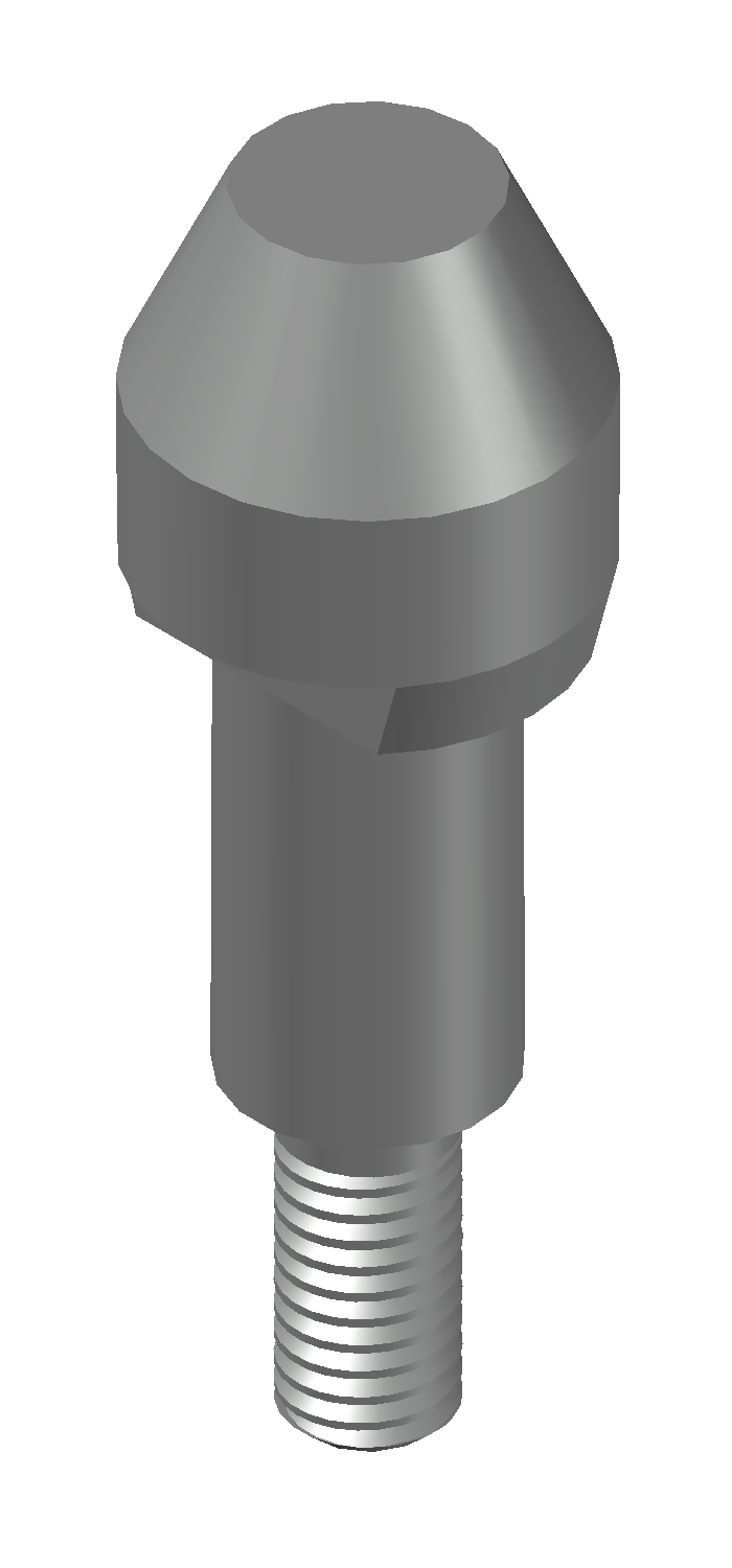
Phase 10 - External turning and threading: facing, roughing, turning of the external profile (upper conicity, diameter 16, lower diameter), M6 threading, and parting off. This phase groups all surfaces of revolution to maximize concentricity in a single setup.
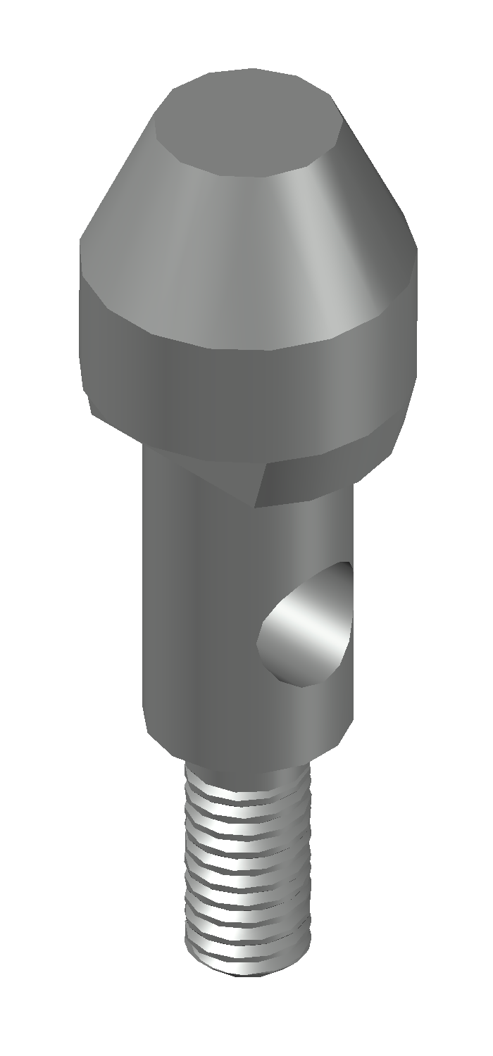
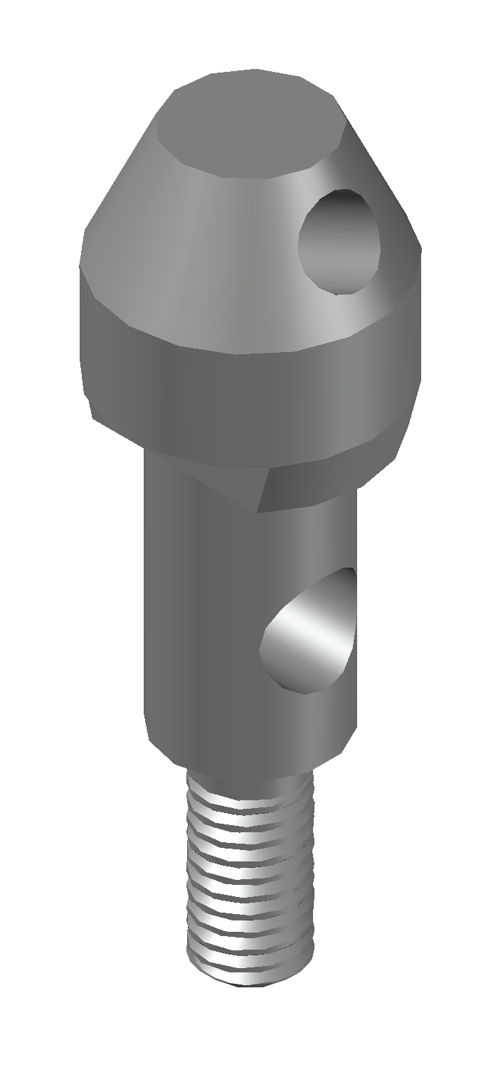
Phase 20 - Milling and transverse and inclined machining: pass-through drilling diameter 6.5 mm and creation of the M6 threaded hole inclined at 25° relative to the vertical axis.

Choice of turning parameters

Facing and roughing
For roughing, obtaining tight tolerances and high surface quality is not fundamental; rather, it's necessary to find the right compromise between machining speed and limiting tool wear.
Parameter	Value	Reason
Cutting speed (Vc)	120 m/min	Intermediate value recommended by reference tables for machining austenitic stainless steels with coated carbide inserts. Offers a good compromise between productivity and safeguarding cutting edge life.
Feed rate (a)	0.20 mm/rev	Working AISI 316, a substantial feed is crucial to allow the cutting edge to pass below the layer work-hardened by the previous pass and thus preserve the tool.
Depth of cut (p)	0.8 mm	Depth of cut necessary to leave enough machining allowance to allow finishing.

Finishing
For finishing, parameters must be adapted so as to meet the tolerance and surface quality constraints of the finished part.
Parameter	Value	Reason
Cutting speed (Vc)	150 m/min	A targeted increase in cutting speed on the final pass locally heats the chip and prevents built-up edge phenomena, guaranteeing the high surface quality required.
Feed rate (a)	0.05 mm/rev	Feed must be reduced to a minimum to meet requested surface finish using a standard size insert (0.4 mm).
Depth of cut (p)	0.2 mm	Equal to the residual machining allowance after roughing.

Parting off
Parameter	Value	Reason
Cutting speed (Vc)	70 m/min	Reduced to limit vibrations on a thin-blade tool and avoid overheating the cutting edge trapped in the cut groove.
Feed rate (a)	0.05 mm/rev	Feed must be low to mitigate radial thrust and prevent insert breakage, while still guaranteeing chip removal.
Depth of cut (p)	3 mm	In parting off, cutting edge width geometrically corresponds to depth of cut, as it defines the width of the removed chip. A standard 3 mm wide insert is chosen to guarantee robustness.

Formulas and calculations

Parameter	Formula	Calculation for facing and roughing	Calculation for finishing	Calculation for parting off
Number of revs (n)	n=1000VcD	Approximated 2100 revs/min	Approximated 3000 revs/min	Approximated 1200 revs/min
Feed velocity (Vf)	Vf=an	420 mm/min	150 mm/min	60 mm/min
Chip cross-section (S)	S=pa	0.16 mm2	0.01 mm2	0.15 mm2
Cutting force (Fc)	Fc=KiSr(p5a)hassuming specific cutting pressure for austenitic inox Ki=2800 N/mm2 and material coefficient r=0.803 and chip slenderness exponent h=0.16.	620 N	67 N	900 N
Cutting power (P)	P=FcVc60000	1.24 kW	0.17 kW	1.05 kW
Machine power (Pm)	Pm=P assuming machine efficiency =0.7.	1.77 kW	0.24 kW	1.5 kW
Machining time (t)	t=LVf considering pass length L = 50 mm (obtained by adding overtravel to total part length).	0.12 min (approx. 7 s)	0.33 min (approx. 20 s)	0.17 min (approx. 10 s)

Choice of lathe

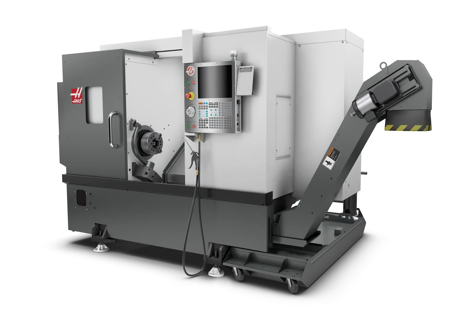
Binding ourselves to the obtained turning parameters, requested tolerances, and necessary surface quality, we chose the Haas ST-10 CNC lathe. This is because it guarantees sufficient efficiency for the 500 pcs/month batch without the financial burdens of higher-end machinery, which would not be justified by actual production needs.

Haas ST-10

Spindle power	11.2 kW
Max speed	6000 revs/min
Indicative price	€ 50000

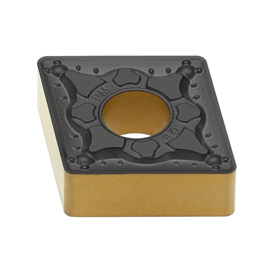
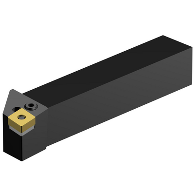
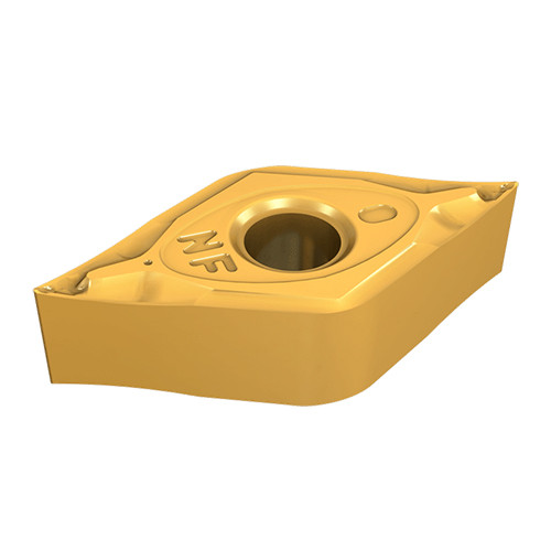
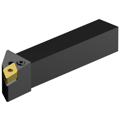
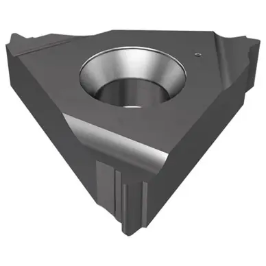
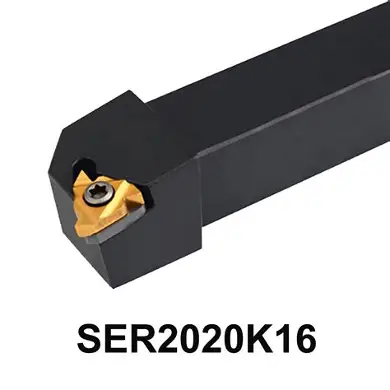
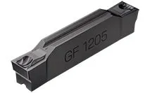
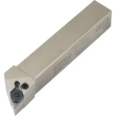
Choice of tools

Tool choice was influenced by:

AISI 316 Stainless Steel (marked tendency to work-harden, low thermal conductivity, and propensity to sticking);
lathe turret (houses 2525 mm shanks);
machining operations to be performed;
turning parameters.

Facing and roughing phase
The difficulty lies in removing material in a stable manner, overcoming the work-hardened layer without making the part vibrate.
Image	Tool	Characteristics	Reason
	Insert CNMG 120404-PM	Nose radius 0.4 mm. 80° (C) rhombic insert, with neutral clearance (N) making it reversible (4 usable cutting edges). PM format (Pre-machining) with positive chipbreaker and PVD coating.	On such a small diameter (diameter 18), a 0.4 mm nose radius ensures a softer cutting action and better chip control. Thanks to the PM format it cleanly shears Inox without overheating it.
	Toolholder PCLNR 2525M12	Rectangular section shank 2525 mm. Positions insert with 95° approach angle (KAPR).	Ideal for selected lathe turret. This approach angle allows the tool to perform both initial facing and longitudinal turning, discharging cutting forces parallel to lathe spindle axis (axial forces), preserving drive head bearings.

Finishing phase
The difficulty lies in meeting given tolerances and surface finish.
Image	Tool	Characteristics	Reason
	Insert DNMG 150404	55° (D) rhombic insert, 0.4 mm nose radius (04).	The 55° shape allows reaching complex plug profile without interference. The 0.4 mm radius, combined with a very slow feed (0.05 mm/rev), generates a near-mirror surface, perfect for gasket seat.
	Toolholder PDJNR 2525M15		Uses the same rigid lever lock (P) as the roughing toolholder, but oriented to maximize clearance space for the lathe turret during profiling movements on small components.

Threading phase
Image	Tool	Characteristics	Reason
	Insert 16ER 1.00 ISO	External threading insert (E), right-hand cutting edge (R), with 60° profile (metric standard M). Carbide cutting edge material with coating.	Specific insert for 1 mm threads. Cutting edge material designed to resist wear on stainless steels.
	Toolholder SER 2020K16	Shank 2020 mm (He B). N.B. Requires insertion of 5 mm calibrated shims.	Specific for external threads. Functional width and geometry allow approaching cylinder shoulder in complete safety during rapid disengagement at the end of every cycle pass, avoiding collisions.

Parting off phase
Image	Tool	Characteristics	Reason
	Parting off insert in TIAIN coated carbide, width 3 mm and 5° inclined cutting edge	Housed at blade tip. In carbide. TIAIN coating.	Carbide and specific coating are necessary to machine stainless steel in question.
	Tool-holder block with 2525 mm shank and parting off blade with internal coolant supply	2525 mm section shank. Internal coolant supply.	Chosen with 2525 mm shank to be compatible with the lathe turret. Internal supply is crucial to cool and lubricate the blade and eject chip from the narrow 3 mm groove being formed.

Choice of milling parameters

Wing housing dimensions
Width	16 mm
Height	3 mm
Depth	3 mm

Wing housing
Parameter	Value	Reason
Cutting speed (Vc)	70 m/min	Recommended value for milling austenitic stainless steels with carbide tools, to avoid premature thermal wear.
Cutter diameter (D)	3 mm	Chosen equal to housing height to be able to achieve vertical dimension in a single pass, optimizing times.
Number of teeth (z)	4	Guarantees good rigidity, which is a fundamental parameter for such a thin bit.
Feed per tooth (az)	0.015 mm/tooth	Commensurated with a small-sized cutting edge to avoid breakage, yet guaranteeing it penetrates material.
Depth of cut (p)	3 mm	Corresponds to the created housing depth.

Formulas and calculations

Parameter	Formula	Calculation
Number of revs (n)	n=1000VcD	Approximated to 7400 revs/min
Feed per rev (a)	a=azz	0.06 mm/rev
Feed velocity (Vf)	Vf=azzn	444 mm/min
Angle ()	cos()=D2-pD2	180° (tool is working at 100% engagement)
Max chip thickness (smax)	smax=azsin()	3 mm (corresponds to cutter diameter)
Max chip cross-section (Smax)	Smax=smaxb with b=3 mm from previous considerations	0.045 mm2
Cutting force (Fc)	Fc=KiSmax assuming specific cutting pressure for austenitic inox Ki=2800 N/mm2 and material coefficient r=0.803	126 N
Cutting power (P)	P=FcVc60000	0.147 kW
Machine power (Pm)	Pm=P assuming machine efficiency =0.7	0.21 kW
Machining times (t)	t=LVf2 considering L = 22 mm (obtained adding to 16 mm length, cutter diameter and overtravel); result must be multiplied by 2 because this machining is performed 2 times (one per side).	0.10 min (approx. 6 s)

Choice of milling machine

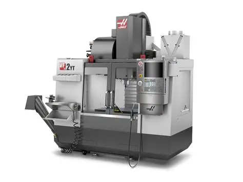
The choice fell on the Haas VF-2 4-axis CNC vertical machining center since it features sufficient max speed (required regime is not supported by lower-end machines) and is highly efficient being numerical control and allowing drilling operations simply by changing insert.

Haas VF-2

Spindle power	22.4 kW
Max speed	8100 revs/min
Indicative price	€ 65000

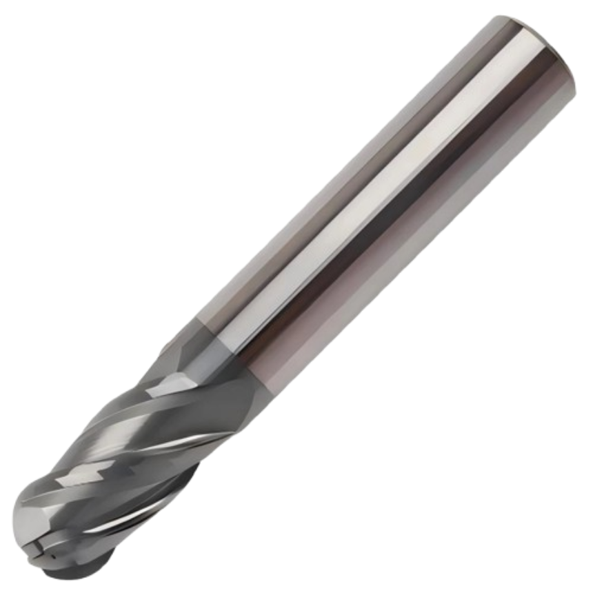
Choice of tools

Image	Tool	Characteristics	Reason
	Solid carbide end mill with 4 flutes diameter 3 mm with TIAIN coating	Made from solid carbide TIAIN coating 4-flute geometry with center cutting edge.	Such a thin tool working at high regimes needs the strength of solid carbide. TIAIN coating serves to increase tool characteristics at high temperatures, typical for machining the chosen inox steel, which has low thermal conductivity. 4 flutes maximize the tool's central web thickness, ensuring robustness. The center cutting edge is fundamental to plunge vertically into solid material.

Choice of drilling parameters

Transverse hole
Parameter	Value	Reason
Cutting speed (Vc)	45 m/min	Optimal value to not overheat austenitic stainless steels machined with carbide drills.
Feed rate (a)	0.08 mm/rev	Sufficient feed for the drill to penetrate beneath the work-hardened layer.

Inclined hole (pre-hole)
Parameter	Value	Reason
Cutting speed (Vc)	45 m/min	See above.
Feed rate (a)	0.06 mm/rev	Slightly reduced compared to above to compensate for lower rigidity of a smaller diameter drill.

Tapping
Parameter	Value	Reason
Cutting speed (Vc)	10 m/min	Tapping involves very low speeds to avoid thread breakage due to high adhesion forces.
Feed rate (a)	1.0 mm/rev	Bound value: must correspond to thread pitch.

Hole dimensions

	Transverse hole	Inclined hole (pre-hole)	Inclined hole (pre-hole)
Diameter	6.5 mm	5 mm	6 mm
Depth	10 mm (pass-through)	6 mm	6 mm

Formulas and calculations

Parameter	Formula	Calculations for the transverse hole	Calculations for the pre-hole	Calculations for tapping
Number of revs (n)	n=1000VcD	Approximated 2200 revs/min	Approximated 2900 revs/min	Approximated 500 revs/min
Feed velocity (Vf)	Vf=fn	176 mm/min	174 mm/min	500 mm/min
Chip cross-section (S)	S=aD4	0.13 mm2	0.075 mm2	1.5 mm2
Tearing coefficient (Ks)	Ks=5Rm considering Rm as the mid value of the range for the chosen stainless steel(600 N/mm2)	3000 N/mm2	3000 N/mm2	3000 N/mm2
Cutting force (Fc)	Fc=KsS	390 N	225 N	4500 N
Cutting power (P)	P=FcVc60000	0.29 kW	0.17 kW	0.75 kW
Machine power (Pm)	Pm=P assuming machine efficiency =0.7	0.41 kW	0.24 kW	1.07 kW
Machining times (t)	t=LVf	0.11 min (approx. 6 s)	0.05 min (approx. 3 s)	0.01 min (approx. 1 s)

Choice of drill

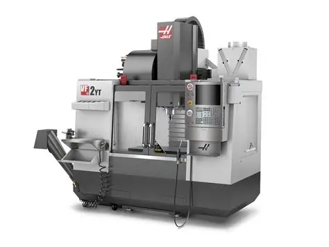
The presence of an inclined hole precludes the use of a traditional pillar drill because it would require additional surface preparation processes, use of drill jigs, and increased labor times. Therefore, it was decided to use the same machine as for milling, simply by changing tools. In this way, money is saved both in terms of purchasing the machine (purchase costs are amortized between the two processes)

Haas VF-2

Spindle power	22.4 kW
Max speed	8100 revs/min
Indicative price	€ 65000

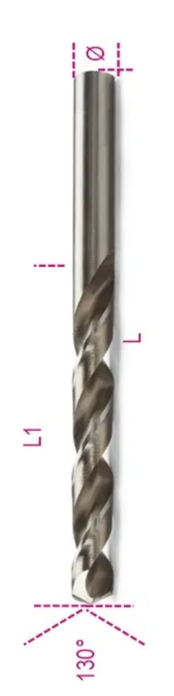
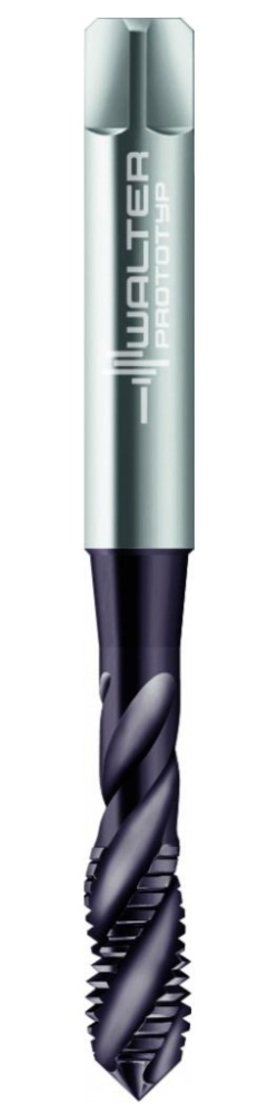
Choice of tools

Transverse hole and inclined hole (pre-hole)
Image	Tool	Characteristics	Reason
	HSS-Co 5% twist drill (6.5 mm and 5.0 mm diameter respectively for transverse hole and pre-hole)	5% cobalt increases wear resistance and hot hardness. 130° point angle.	AISI 316 being poorly conductive tends to overheat during machining, so maintaining tool properties as temperatures rise is a crucial factor. This angle offers good initial penetration, reducing axial thrust effort.

Tapping
Image	Tool	Characteristics	Reason
	HSS-E PM machine tap (M6)	High toughness and torsional resistance thanks to powder metallurgy manufacturing. Helical flute	High tool mechanical properties prevent its breakage inside the hole, a particularly critical phenomenon for the chosen stainless steel. The helical flute is fundamental for blind holes as it allows evacuating chips outside the hole.

Lubricoolant cooling

For machining AISI 316 Stainless Steel, the choice and application methodology of the lubricoolant fluid must directly respond to material criticalities: very low thermal conductivity (which concentrates heat on tool) and strong tendency for chip to work-harden and adhere.

	Turning, milling and drilling	Tapping
Lubricoolant type	High concentration emulsion (water and oil) (typically between 8% and 12% mineral or synthetic additivated base).	Neat cutting oil or specific tapping pastes for Inox.
Reason	Water component is vital to drop generated high temperatures. High oil percentage provides lubricating power needed to make chip slide and avoid built-up edge phenomenon.	Being a very low speed operation with high adhesion and friction forces in a blind hole, standard emulsion is often insufficient.
Application methodology	High pressure and precision: Jet must be delivered abundantly and aimed exactly at cutting interface between insert and part. Continuous and preventive delivery: Liquid must flood cutting edge before it contacts material and maintain constant flow. For parting off and drilling, internal supply is used: used drill has internal lubrication holes where high pressure lubricoolant fluid is injected.	HSS-E tap coating is specifically designed to retain lubricant in its microporosities.
Reason	Intermittent or delayed delivery would cause thermal shocks on carbide insert, generating micro-cracks. High pressure liquid forcefully pushes chips up flute grooves, preventing them from compacting at bottom and causing tool breakage.	Lubricant present in microporosities prevents microwelding.

Initial setup and CNC lathe preparation

Before starting the production batch, the following setup operations must be performed:

Bar loading and adjustment: Inserting Ø18 mm AISI 316 Stainless Steel bar into spindle and adjusting collet pressure, verifying correct ejection via hydraulic bar feeder.
Bar puller setup: A bar puller must be tooled in the turret. This acts as a physical stop and ensures that, at each cycle end, the bar feeder advances the blank by the exact amount needed for the next part (equal to 47.65 mm finished length, plus 3 mm parting tool thickness and 1 mm facing machining allowance).
Tool offsetting: Each tool must be zeroed via automatic presetting to communicate length and nose radius of each insert to numerical control. This allows the machine to calculate exact compensations and toolpaths.
Part origin zeroing (G54): Part zero (Z=0) is defined, being set on front face, following facing, creating a reliable reference plane for all axial dimensions.
Lubricoolant management: Lubricoolant nozzles are arranged to aim exactly at the cutting area of every single tool.

Initial setup and CNC machining center preparation

The following operations are required before starting production batch:

Fixture and part placement: Mounting a concentric clamping system (precision collet chuck) directly on the 4th axis rotary table. The plug, coming from the lathe, is clamped by grabbing it on the cylindrical portion.
Part origin (G54) and center of rotation zeroing: Via a 3D probe, exact cylinder center for X and Y axes is found, and zero (Z=0) is established on the upper face of the conical head. It is fundamental that numerical control knows the exact distance between part origin and center of rotation (COR) of the 4th axis.
Tool zeroing in magazine: Measuring tool length and radius, via on-machine laser presetting. Perfect cutter zeroing is crucial to respect dimensions and tolerances.
Lubricoolant management and control: Lubricoolant nozzles are specifically set to ensure proper functioning. Furthermore, liquid composition itself is verified.

Time calculation

Time analysis for cylindrical plug production is divided into setup times (initial machine setup, not dependent on single part but amortized over batch) and machining times (active machine cycle to make a single component).

Setup times analysis: Setup is performed by an operator once before starting the batch. Following values are standard industrial estimates for qualified operators on modern CNC machines:
Haas ST-10 CNC Lathe

Bar loading and collet adjustment: ~10 min
Bar puller and bar feeder setup: ~5 min
Tool offsetting: ~10 min
Part origin zeroing: ~2 min
Lubricoolant management: ~3 min
Total estimated lathe setup: ~30 minutes. Dividing this time by 500-piece batch, impact on single piece is only 0.06 minutes/piece.

CNC Machining Center

Collet chuck placement on CNC indexer (4th axis): ~20 min
Origin and center of rotation (COR) zeroing: ~10 min
Tool offsetting: ~10 min
Lubricoolant management: ~5 min
Total estimated milling machine setup: ~45 minutes. Dividing by 500 pieces, impact is 0.09 minutes/piece.

Machining times analysis (machine time): These times are based on formulas t=LVf indicated in the routing sheet, which calculates pure cutting time. To get real piece time, a markup (usually 30-40%) must be added to include rapid movements, tool changes, and load/unload.

Turning and parting off (Haas ST-10)

Facing and roughing: 0.12 min (7 sec)
Profile finishing: 0.33 min (20 sec)
External M6 threading: ~0.15 min (Estimate: G76 multi-pass cycles)
Parting off: 0.17 min (10 sec)
Total lathe cutting time: 0.77 min.
Estimated idle time (tool changes, approaches, bar feeder): ~0.30 min
Estimated part time (Lathe): ~1.07 minutes.

Milling and drilling (Haas VF-2)

Wing housing milling (Ø3 cutter, two sides): 0.10 min (6 sec)
Transverse pass-through drilling Ø6.5 (10 mm): 0.11 min (6 sec)
Inclined blind pre-hole Ø5 (6 mm): 0.05 min (3 sec)
M6 Tapping: 0.01 min (1 sec)
Total milling machine cutting time: 0.27 min.
Estimated idle time (4th axis rotations, 3 tool changes, manual part load/unload on collet): ~0.80 min.
Estimated part time (milling machine): ~1.07 minutes.

Total process time: To make entire 500-piece batch, overall time required of shop will be:

Overall machine setup: 30 min (Lathe) + 45 min (Machining Center) = 75 minutes (1 hour and 15 min).
Machining time (1 piece): 1.07 min (Lathe) + 1.07 min (Machining Center) = 2.14 minutes / piece.
Machining time for batch (500 pcs): 2.14 min * 500 = 1070 minutes (17 hours and 50 minutes).
Absolute total time (setup + machining): 75~min+1070~min=1145 minutes, meaning just over 19 working hours. This proves that the monthly batch will engage shops for almost two and a half effective work shifts.

1. Machinery Amortization (5-year Plan)

Amortization transforms machine purchase cost into an hourly cost. Considering standard industrial use on a single shift (about 1600 annual working hours), following values are obtained:

Haas ST-10 CNC Lathe:

Indicative price: € 50,000.
Annual amortization quota (5 years): € 10,000 / year.
Machine hourly cost: € 10,000 / 1600 hours = 6.25 €/h.

Haas VF-2 CNC Machining Center:

Indicative price: € 65,000.
Annual amortization quota (5 years): € 13,000 / year.
Machine hourly cost: € 13,000 / 1600 hours = 8.12 €/h.

2. Machine Usage Cost for Batch (500 pcs)

Applying operational timings defined for batch:

Lathe Engagement: 30 setup minutes + (1.07 minutes/piece * 500 pieces) = 565 minutes (9.42 hours).

Lathe amortization cost for batch: 9.42~h6.25€/h=58.87€.

Milling Machine Engagement: 45 setup minutes + (1.07 minutes/piece * 500 pieces) = 580 minutes (9.67 hours).

Milling machine amortization cost for batch: 9.67~h8.12€/h=78.52€.

Amortization impact on single piece: (58.87€+78.52€)/500= 0.27 €/piece.

3. Raw Material Cost

Components are made starting from an extruded and drawn Ø18 mm AISI 316 (1.4401) Stainless Steel bar.

Blank length per piece: 47.65 mm (finished dimension) + 3 mm (parting thickness) + 1 mm (facing machining allowance) = approx. 52 mm.
Blank volume: (9mm)252mm13.23cm3.
Blank weight: Considering specific weight of 8~g/cm3, each piece consumes about 106 grams of stainless steel.
Cost estimate: Assuming a commercial cost for AISI 316 bar of about 6.00€/kg, blank cost is 0.106kg6.00€/kg= 0.64 €/piece.

4. Direct Labor Cost

The total time to make the entire batch is 1145 minutes, equal to about 19 working hours. Assuming a standard cost for a specialized CNC operator of 35.00 €/hour:

Batch labor cost: 19.08 hours35.00€/h=667.80€
Labor impact on single piece: 667.80€/500= 1.34 €/piece

5. Tooling and Electrical Energy Cost

AISI 316 has poor thermal conductivity and tends to overheat and work-harden very rapidly, leading to accelerated wear of carbide inserts and HSS-E taps. Moreover, machinery requires electrical power to operate (11.2 kW and 22.4 kW spindles).

Lump-sum tool/fluid consumption estimate: Given tough material, an insert consumption and drill/cutter wear of about 0.60 €/piece is estimated.
Energy estimate: About 0.15 €/piece.
Total tooling and energy: 0.75 €/piece.

Final Production Cost Summary (Single Plug)

Raw Material (AISI 316 Ø18)	0,64 €	21,3%
CNC Operator Labor	1,34 €	44,7%
Tooling, Fluids and Energy	0,75 €	25,0%
Total Production Cost	3,00 € / pezzo	100%

Routing sheet

Drawing	Phase no.	Subphase no.	Operation Description	Machine	Equipment
	10	10.1	Profile facing and roughing	CNC Lathe Haas ST-10	Insert CNMG 120404-PM Tool-holder PCLNR 2525M12
		10.2	Profile finishing		Insert DNMG 150404 Tool-holder PDINR 2525M15
		10.3	M6 external threading		Insert 16ER 1.00 ISO Tool-holder SER 2020K16
		10.4	Parting off		Parting off insert in TIAIN coated carbide, 3 mm width and 5° inclined cutting edge Tool-holder block with 2525 mm shank and parting blade with internal coolant supply
	20	20.1	Wing housing milling	4-axis CNC vertical machining center Haas VF-2	Solid carbide end mill with 4 flutes Ø3 mm with TIAIN coating
		20.2	Transverse pass-through hole drilling		HSS-Co 5% twist drill 5.0 mm diameter
		20.3	Blind inclined pre-hole		Punta elicoidale HSS-Co 5% di diametro 5,0 mm
		20.4	Tapping		HSS-E PM machine tap (M6)

Metrological controls

As indicated in the phase definition chapter, main tolerances have been extrapolated from drawing, for which measuring instruments capable of appreciating them are reported.

analog decimal caliper
micrometer with range up to 25 mm
thread quality control with optical profilometer to verify pitch and correct profile execution
analog decimal caliper
analog decimal caliper
control with thread gauge