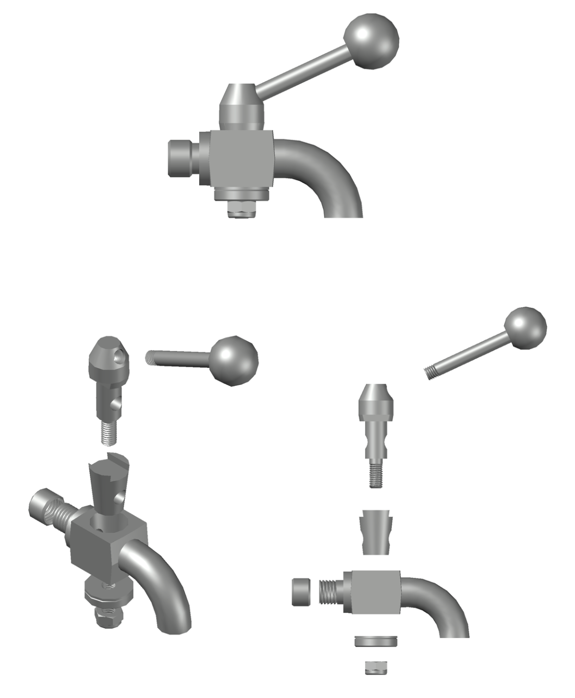
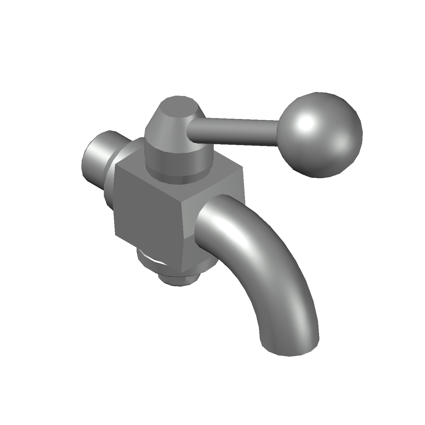
The component under study is a taper plug sampling cock (also known as a taper plug valve), designed for industrial and food-grade applications (particularly in the wine sector) thanks to the high corrosion resistance guaranteed by AISI 316 stainless steel

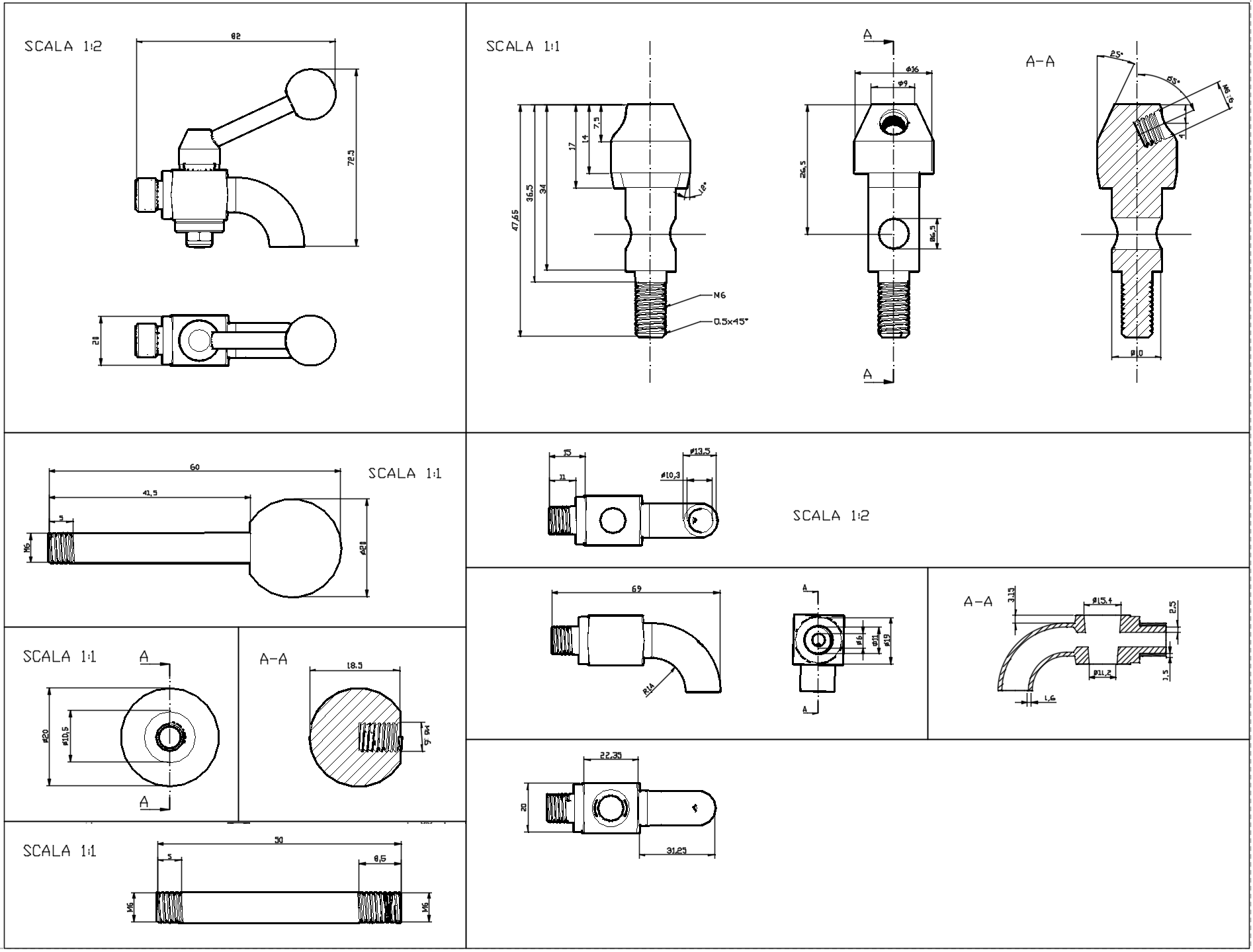
Below the drawings of the finished product:

Below are the dimensions of the assembly

Foundry - Valve Body

The dimensions of the part as it leaves the foundry, ready for machining:

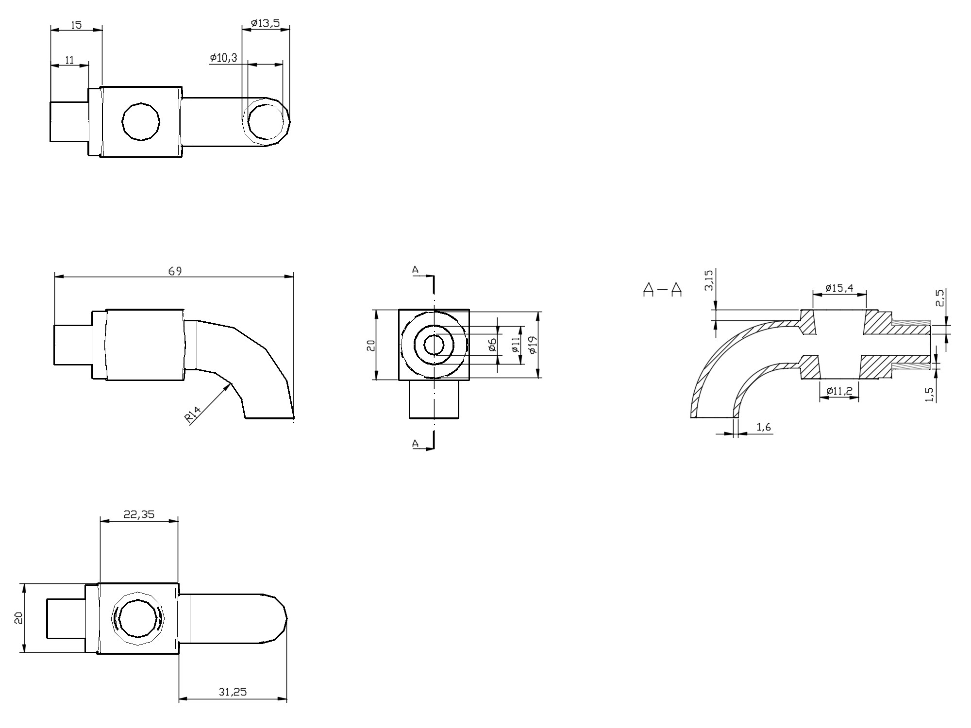
Chamfers not represented

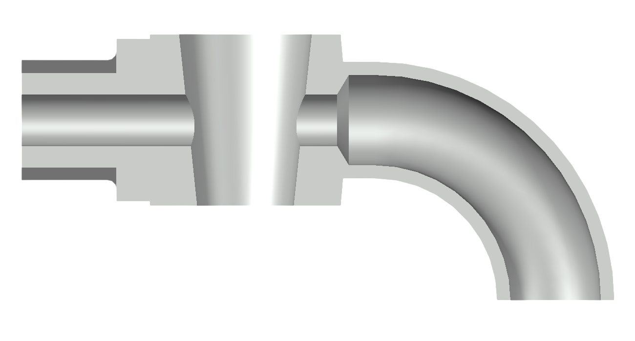
Main characteristics of the part

For the purposes of choosing and studying the casting process, the main characteristics of the part are reported analytically:

monthly production of 500 pieces

relatively simple geometry

general machining tolerances and tolerance only on the internal conical surface for assembly equal to 0.05-0.2 mm

general surface finish Ra6 m, no special finishes

limited machining required at the interfaces (threading for installation)

Choice of process

Considering a monthly production of 500 pieces, therefore repeatable, permanent mold or pattern casting processes can be considered, which allow for:

better mechanical properties,

better quality in terms of dimensional accuracy and surface finish and

higher productivity, thanks to reduced times for molding and for solidification and cooling.

Among the permanent mold processes, we exclude die casting both by gravity and by pressure, since the alloy of which the piece is made is stainless steel: a steel die would not withstand the melting temperature of such a material, it would be necessary to resort to complex solutions such as making the die in a material with a high melting point, designing a cooling system for it and/or the use of special refractory substances with which to coat the area of the die in contact with the molten steel.

The pressure die-casting system even more so, from an economic point of view, would not be convenient due to the additional costs of the cold chamber or hot chamber machine, which are difficult to amortize given the required productivity (500 pieces/month).

The choice therefore falls on one of the techniques with a permanent pattern, in particular shell-molding.

We also exclude investment casting due to the greater slowness of the process against a higher quality not required for the piece in question.

The shell-molding process is suitable for making our part.

On the one hand, it implies an increase in costs for the purchase of machinery capable of injecting the molding material between the pattern plate and the cover and for the energy necessary to heat and polymerize the resin, furthermore the material used cannot be recovered but the waste of material is less than in sand molding, given the reduced thickness of the shells; the process is also easily automatable, the surface finish and dimensional accuracy are very good, which fall within the aforementioned tolerances, the molding material must have high flowability and be very permeable to avoid the blowhole defect. The weight of the piece is much less than the maximum limit for this process (up to 30 kg), therefore it is a good candidate to be chosen for making the part.

Choice of parting line

The plane of symmetry has no undercuts and is chosen as the parting line.

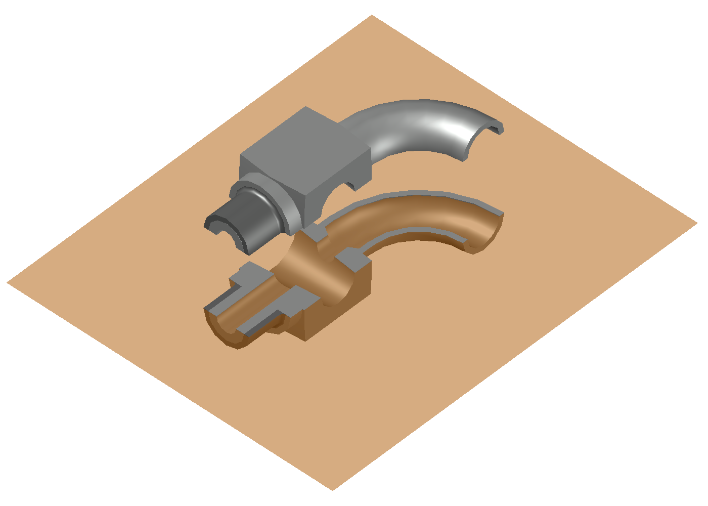
Machining allowances

Since there are no undercuts, the machining allowance is provided only in the interface area where a thread with a relief groove will have to be executed, with the exception of the internal cavities which are generated through a core treated in the appropriate section.

Regarding the parts to be subsequently machined, the part does not have any dimension greater than 100 mm, therefore Santochi recommends a machining allowance of 1.5 mm.

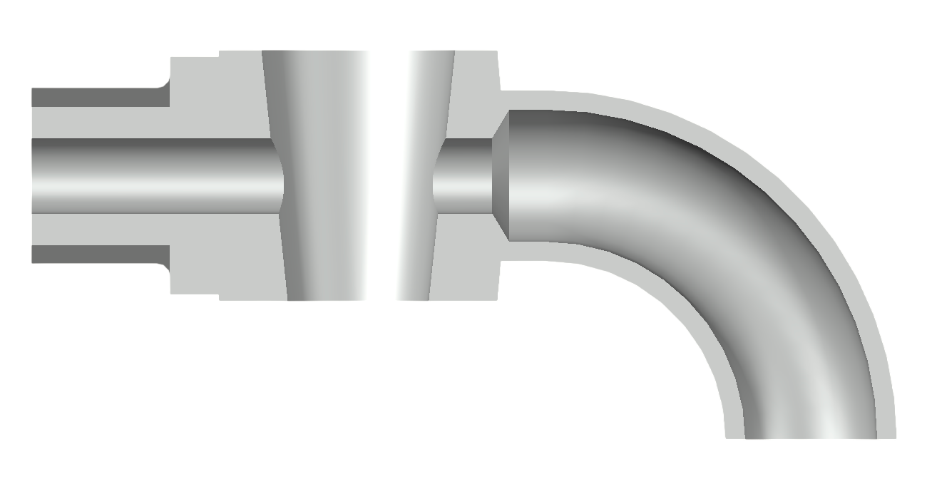
Pattern simplification

Elimination of holes

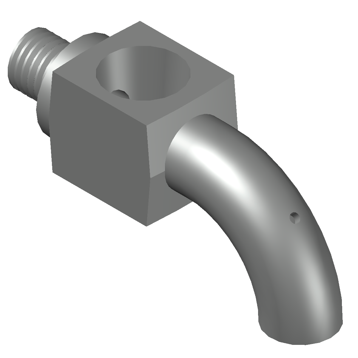
The internal cavities that are undercut are made using a core in the dedicated section.

Regarding the hole of the piece, such a thickness in a part of the shell, even if it were achievable, would make the mold fragile, with possible deformations or fractures during the solidification phase. Furthermore, if it were necessary to make a core this would entail costs and an increase in time, making it not convenient compared to making the holes a posteriori, also given the small drilling diameter.

Shrinkage

To take into account the contraction during the solidification phase and the cooling phase, the pattern plate is oversized considering the linear shrinkage of the stainless steel equal to 2 percent from the pouring temperature to room temperature.

Since it is a small steel casting, the average linear shrinkage coefficient (hereinafter ) is about 2%. Therefore the scale factor (s) is calculated as follows, taking into account the shrinkage of an edge of unit measure:

1:(1-)=s:1

s=1/(1-)=1/(1-0.02)=1.0204

Therefore, the dimensions of the pattern plate must be increased by approximately 2% compared to the nominal dimensions of the part, in order to compensate for the contraction of the material during cooling.

For reasons of speed, the dimensions of the drawing are to be intended with a shrink rule, meaning the drawing is not resized to account for shrinkage, but contains the nominal dimensions.

Draft angles

Given that we use a permanent pattern and a transitory shell, draft angles are to be provided for the molding operation (shell creation). The draft angle depends on the friction angle between the metal of the pattern plate (reduced thanks to the use of any parting powders) and the sand for shell-moulding, and corresponds to 1 degree.

The part is built by cylindrical and truncated-conical revolution surfaces which therefore do not require draft angles, and by flat surfaces perpendicular to the parting plane highlighted

Cores

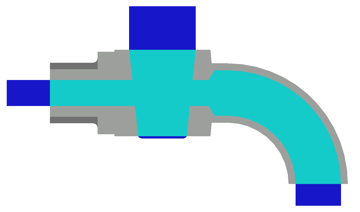
Choice of process

Considering the volumes that economically justify the use of shell-moulding, the advantages already listed remain.

Given the casting procedure chosen for the piece, the choice of the molding technique for core necessarily falls on the techniques in transitory mold. In particular, as regards the core, for homogeneity with the rest of the piece and for the observations on quality and cost-effectiveness made in the point on the choice of the process, it is decided to use the shell molding technique.

Core design

In the figure you can see the dimensioned drawings of the metal core boxes and of the core. The parting line coincides with the symmetry plan.

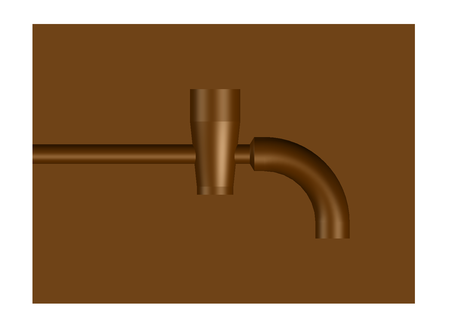
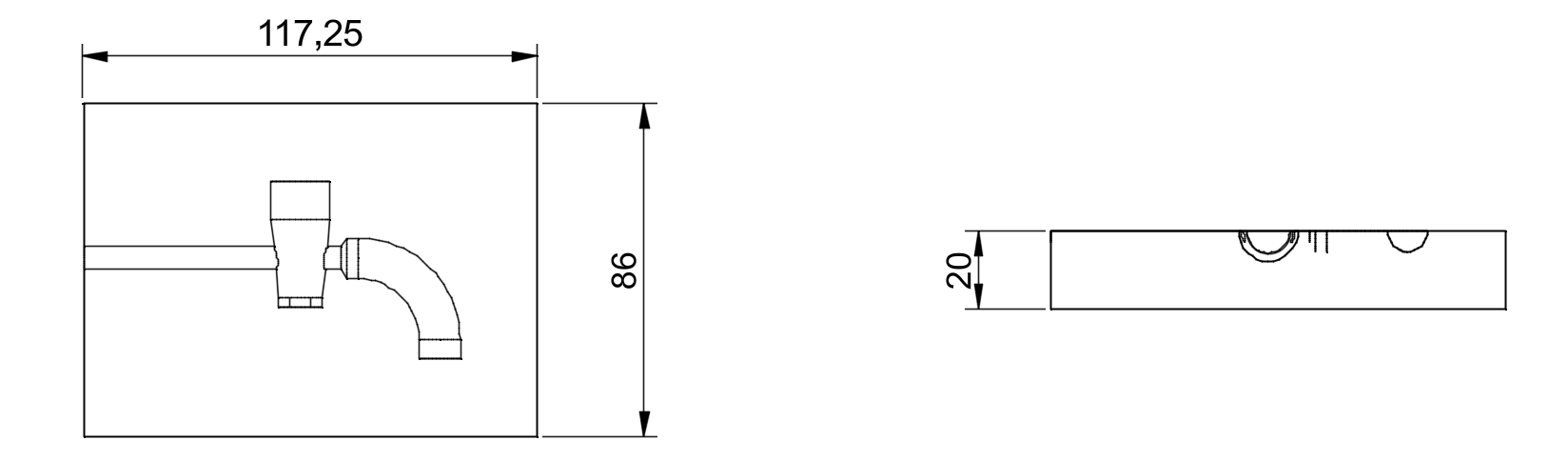
The values of the cylindrical core prints taken from company literature are 10 mm. To give maximum stability, 3 core prints are provided since the internal cavity is formed by two intersecting cavities, while a 0.5 mm diameter corer aids in the removal of the sprue at the end of the process.

Fillet radii

The fillet radii must be introduced at the corners of the mold which can be eroded by the flow of molten steel, therefore the problem exists only for the edges that generate concave angles since in the mold they will be the ones that will generate convex, protruding angles, therefore more subject to erosion.

The chamfers in the drawing of the dimensioned part and of the raw part are represented by fillet radii R=0.5 mm equal to the thickness of the machining allowance.

Directional solidification

Once the more "geometric" problems have been solved and the final shape of the raw part has been defined, to have the final drawing of the pattern plates, any components that aim to minimize foundry defects (feeders, chills, etc.) and the gating system must be designed. Between the two, the solidification of the raw part is analyzed first since the possible addition of feeders changes its geometry and weight, with a consequent increase in filling time, cost of material and energy; furthermore, the gating system can be exploited to generate hot spots and thus modify solidification.

To design any feeders, chills or other components, it is necessary to study the solidification of the raw part, to understand the direction of solidification and the critical areas and then insert the components where necessary. Lacking the gating system, it is assumed that initially the raw part is all at the same temperature. The techniques at our disposal for the study of the solidification of the casting are:

the subdivision of the casting into elementary solids and the calculation of the cooling module of the latter, to then order them and thus deduce the solidification order;

the Heuvers circle method to ensure that there are no interruptions in the flow and not to nullify the contribution of the feeder;

solidification simulation via software starting from the CAD model of the raw part.

Simplified calculation of cooling modules

We proceed with the decomposition of the model into elementary solids. The four modules into which the part is virtually decomposed are all assimilable to a bent bar as in the estimation of the bored cylinder on Santochi, in particular:

1 (orange) cube with conical hole is assimilated to a bored cylinder; the conical hole is approximated to a cylindrical hole, with average dimension of the two bases

M1 = (S1 * S2 ) / 2 / ( S1 * S2) = (13.3 * 4.45) / 2 / (13.3 + 4.45) = 1.82 mm

the calculation is repeated considering also the thickness values at the extremes to evaluate the variability in considering the average value

M1’ = (S1 * S2 ) / 2 / ( S1 * S2) = (13.3 * 3.4) / 2 / (13.3 + 3.4) = 1.45 mm

M1’’ = (S1 * S2 ) / 2 / ( S1 * S2) = (13.3 * 5.5) / 2 / (13.3 + 5.5) = 2.15 mm

Just 16 percent variation, the average value M1 is considered sufficiently conservative, for the purpose of directional solidification.

2 (red) bent bored cylinder

M2 = (S1 * S2 ) / 2 / ( S1 * S2) = (1.6 * 39.11) / 2 / (1.6 + 39.11) = 0.76 mm

3 (green) threaded bored cylinder

M3 = (S1 * S2 ) / 2 / ( S1 * S2) = (2.5 * 11.69) / 2 / (2.5 + 11.69) = 1.02 mm

M3 with machining allowance of 1.5 mm on both sides =1.49 mm

4 (yellow) bored cylinder

M4 = (S1 * S2 ) / 2 / ( S1 * S2) = (4.5 * 6.5) / 2 / (4.5 + 6.5) = 1.23 mm

Given the presence of numerous interface surfaces, the modules could be underestimated but this applies to all four modules, therefore the effect on superficial solidification could be acceptable.

Calculation of cooling modules from CAD

To evaluate the goodness of the approximations, we proceed to the analogous calculation but in an exact manner using the CAD data, exploiting the area and volume calculation tools. At this point we proceed with the calculation of the cooling modules according to the definition:

M=V/SST

where SST is the total heat exchange surface and V is the total volume of the solid. These two data are provided by the CAD; in particular the first is obtained as the sum of the surface areas.

M1cad=1.87 mm

M2cad=0.76 mm

M3cad=1.52 mm

M4cad=1.12 mm

Therefore the solidification order of the geometries is the following: 1 3 4 2

It is therefore verified that, approximately, the solidification proceeds from the outermost parts to the most central ones, except for the threaded input module which will have to be protected by an additional feeder.

Feeder positioning

From the analysis of directional solidification based on the cooling module calculation method (cfr M1, …, M4), there is a single hot spot, therefore a single feeder is sufficient, which must be placed on component 1 with the highest cooling module.

Since M1’’ > M1’, it is decided to place the feeder on the lower side of the tap and consequently the casting will be upside down.

This positioning also improves the coverage (feeding distance) of the outlet pipe, since it is curved downwards.

Heuvers' circle method

To verify that the feeder can correctly feed the casting, the graphical verification of Heuvers' circles is performed.

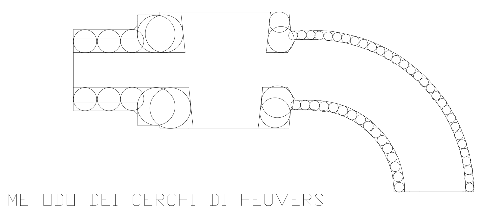
The method applied in the figure provides a positive verification on the hypothesis of feeder placement. Therefore it is not necessary to add machining allowances and then recalculate the cooling modules.

Feeder feeding distance

Since section 4 of the part (curved pipe) has a constant cross-section for its entire length, it is necessary to ensure that there are no bottlenecks that compromise the correct functioning of the feeder.

The feeding distance is:

R=k *S+2.5*S

where k is a coefficient depending on the material =3.5 and S is the wall thickness of the pipe

R1=3.5*2+2.5*2=12~mm>10~mm OK R2=3.5*1.6+2.5*1.6=9.6~mm<31.75 NOT OK

Chills

The feeder covers the inlet part while it seems insufficient for the outlet part.

Among the possible solutions, the positioning of a second feeder is discarded as it seems disproportionate to the potential benefit.

Alternatively, the possibility of increasing the thickness of the pipe was evaluated, but a design change is more onerous than a standard industrialization expedient.

The use of chills to be placed on the outlet side after forming the pattern plates is considered sufficient.

Feeder sizing

Once the solidification of the raw part has been studied, it is necessary to study how to avoid shrinkage cavities through proper sizing of the feeder.

Positioning was already discussed in the dedicated section.

First of all, the module that the feeder must have to be able to solidify last is calculated. Calling Mmax the maximum module of the part, we have:

Mm1.2* Mmax =1.2*1.87=2.244 mm

The preferred choice is open-top to utilize atmospheric pressure to pump the molten metal.

The shape of the feeder is the one that occupies the minimum volume and therefore uses less material and is easy to make. Therefore, the open-top cylindrical feeder is chosen, with H=D, which is easy to mold and is the one that, for the same module, occupies the least volume.

In Santochi:

V=1.18 D

V=179 M

M=0.18 D

At this point, the following values can also be calculated:

Dm=Mm/0.18=12.46 mm

Approximating upwards to a "rounder" value, we set Dm=13~mm. Hm=Dm=13 mm

from which: Vm=(Dm/2)2Hm=1401.75 mm3

feeder surface area, to be used later for verification with Caine's curve:Sm=DmHm+Dm2/4=663.66 mm2.

The height H=D of the feeder also determines the height of the mold and the pattern plate and will influence the length of the sprue.

Feeder neck sizing

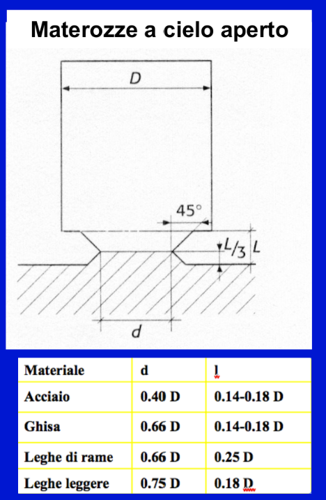
The feeder neck sized following the practice illustrated in the text "Santochi" is shown in the figure of the raw casting.

d=0.4*Dm=5.2 mm since the feeder will be bored due to the presence of the core, the neck will have the shape of a circular ring instead of a circle with an equivalent cross-section. The internal diameter of the circular ring coincides with that of the hole, i.e., 11.2 mm. the external diameter of the circular ring measures dm=dm2+15.42=16.15 mm

Lm=0.17*Dm=2.2~mm

The figure of the raw casting arises from all calculations and represents dimensions of the feeder and neck, gating system, and part with machining allowances and draft angles and fillet radii.

Feeder verification using Caine's method

It must now be verified that the feeder is large enough to provide the metal necessary to avoid the formation of shrinkage cavities. To do this, we use Caine's formula/diagram.

The figure shows the feeder sized in the previous paragraph which is validated using the following diagram parameters:

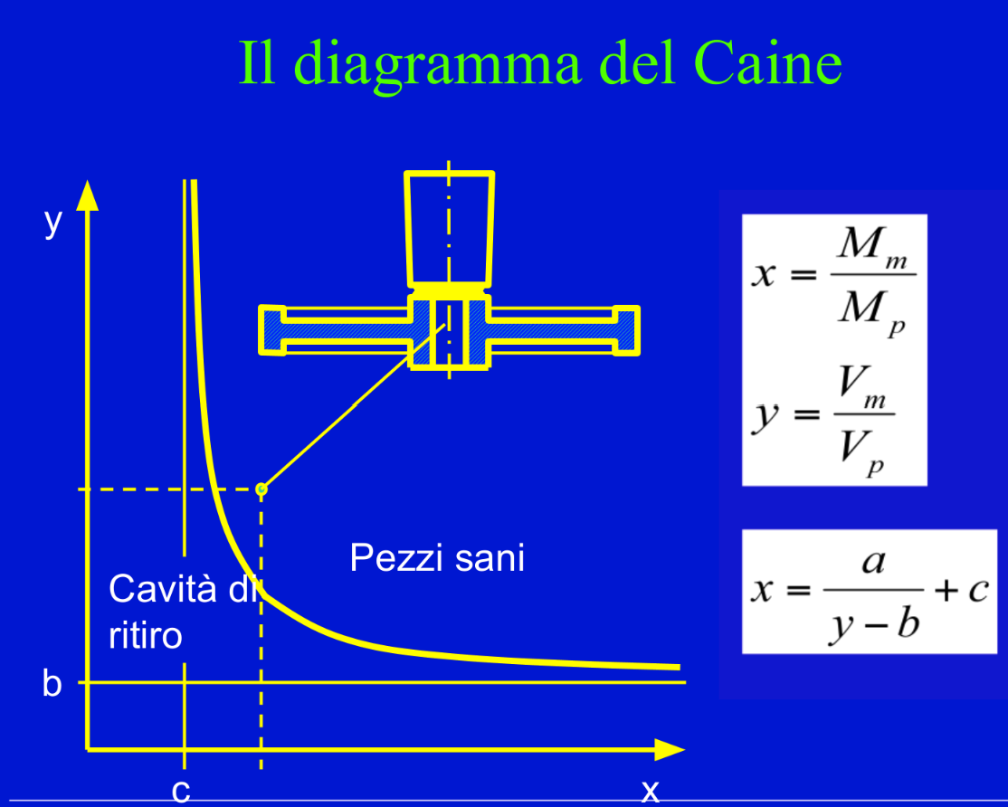
To apply it, it is sufficient to follow the algorithm on page 136 of Santochi. It is therefore necessary to define the parameters to be inserted. The parameters relative to Caine's curve are:

a=0.1 which is a fixed value;

b = 8% since the steel in question is an alloy steel;

c=1 ratio between the heat transfer coefficient of the feeder molding material and the same coefficient for the part molding material (c=1 in the majority of cases; c=0.70.8 for insulated feeders);

For what was said before, an open-top feeder is chosen and, for ease of molding, cylindrical in shape.

The values provided by the CAD software are:

Vp=9850.0272 mm3

Sp=6837.1936 mm2

Mm is the cooling module of the feeder =2.24 mm

Mp is the cooling module of the last section to be protected =1.87 mm

Vm is the volume of the feeder calculated in the specific feeder section

Vp is the volume of the entire part =9850.0272 mm3

For the estimation, the specific Matlab code shown below was developed.

clear; clc; close all;

% --- 1. MATERIAL PARAMETERS (Caine's Equation) ---

% The formula is: X = a / (Y - b) + c

% Below are the classic values for STEEL:

a = 0.1;

b = 0.08;

c = 1.00;

% --- 2. DATA OF YOUR CASTING AND FEEDER ---

V_getto = 9.84; % Volume of the casting [cm³]

A_getto = 68.37; % Surface area of the casting [cm²]

V_mat = 1.4; % Volume of the feeder [cm³]

A_mat = 6.64; % Surface area of the feeder [cm²]

% Calculation of Thermal Modules (M = V / A)

M_getto = V_getto / A_getto;

M_mat = V_mat / A_mat;

% Calculation of coordinates for the point on the diagram

X_punto = M_mat / M_getto; % Module ratio (X-axis)

Y_punto = V_mat / V_getto; % Volume ratio (Y-axis)

% --- 3. GENERATION OF CAINE'S LIMIT CURVE ---

% The volumetric ratio Y must be strictly greater than the lower limit 'b'

Y_curva = linspace(b + 0.01, 1.5, 500);

X_curva = a ./ (Y_curva - b) + c;

% --- 4. PLOTTING THE DIAGRAM ---

figure('Color', 'w', 'Name', 'Diagramma di Caine');

hold on; grid on; box on;

% Defect area (under the curve) and soundness (above)

% For graphic reasons we create a patch for the sound zone

fill([X_curva, max(X_curva), max(X_curva)], [Y_curva, max(Y_curva), min(Y_curva)], ...

[0.85 0.95 0.85], 'FaceAlpha', 0.5, 'EdgeColor', 'none', 'DisplayName', 'Sound Zone (Good Part)');

% Plot of the limit curve

plot(X_curva, Y_curva, 'r-', 'LineWidth', 2.5, 'DisplayName', 'Caine''s Limit Curve');

% Plot of the point for the casting under examination

plot(X_punto, Y_punto, 'ko', 'MarkerFaceColor', 'y', 'MarkerSize', 10, ...

'LineWidth', 1.5, 'DisplayName', 'Casting under Examination');

% --- 5. AXIS CONFIGURATION AND LABELS ---

xlabel('Module Ratio X = M_{mat} / M_{getto}', 'FontSize', 11, 'FontWeight', 'bold');

ylabel('Volume Ratio Y = V_{mat} / V_{getto}', 'FontSize', 11, 'FontWeight', 'bold');

title('CAINE''S DIAGRAM', 'FontSize', 14, 'FontWeight', 'bold');

% Setting axis limits for a better view

xlim([0.5, 2.5]);

ylim([0, 1.5]);

% Adding legend and graphic notes

legend('Location', 'northeast');

% Mathematical check of part soundness

X_limite = a / (Y_punto - b) + c;

if Y_punto > b && X_punto > X_limite

text(X_punto + 0.05, Y_punto, ' CHECK OK: SOUND PART', 'Color', [0 0.5 0], 'FontWeight', 'bold');

else

text(X_punto + 0.05, Y_punto, 'WARNING: SHRINKAGE DEFECT', 'Color', [0.7 0 0], 'FontWeight', 'bold');

end

hold off;

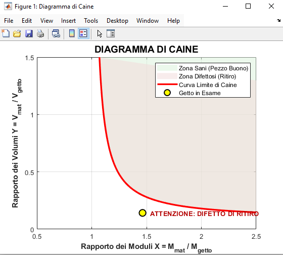
Verification with Caine's diagram shows that the feeder does not have sufficient volume to feed the shrinkage of the entire part.

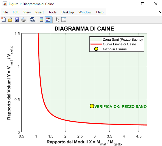
Therefore, we proceed to increase its height to 1.5*Dm instead of 1 so as to leave the sizing of the feeder neck unchanged.

Hm’=19.5 mm

Dm = 13 mm

Vm’=3882.41mm3

Sm’=929.13 mm3

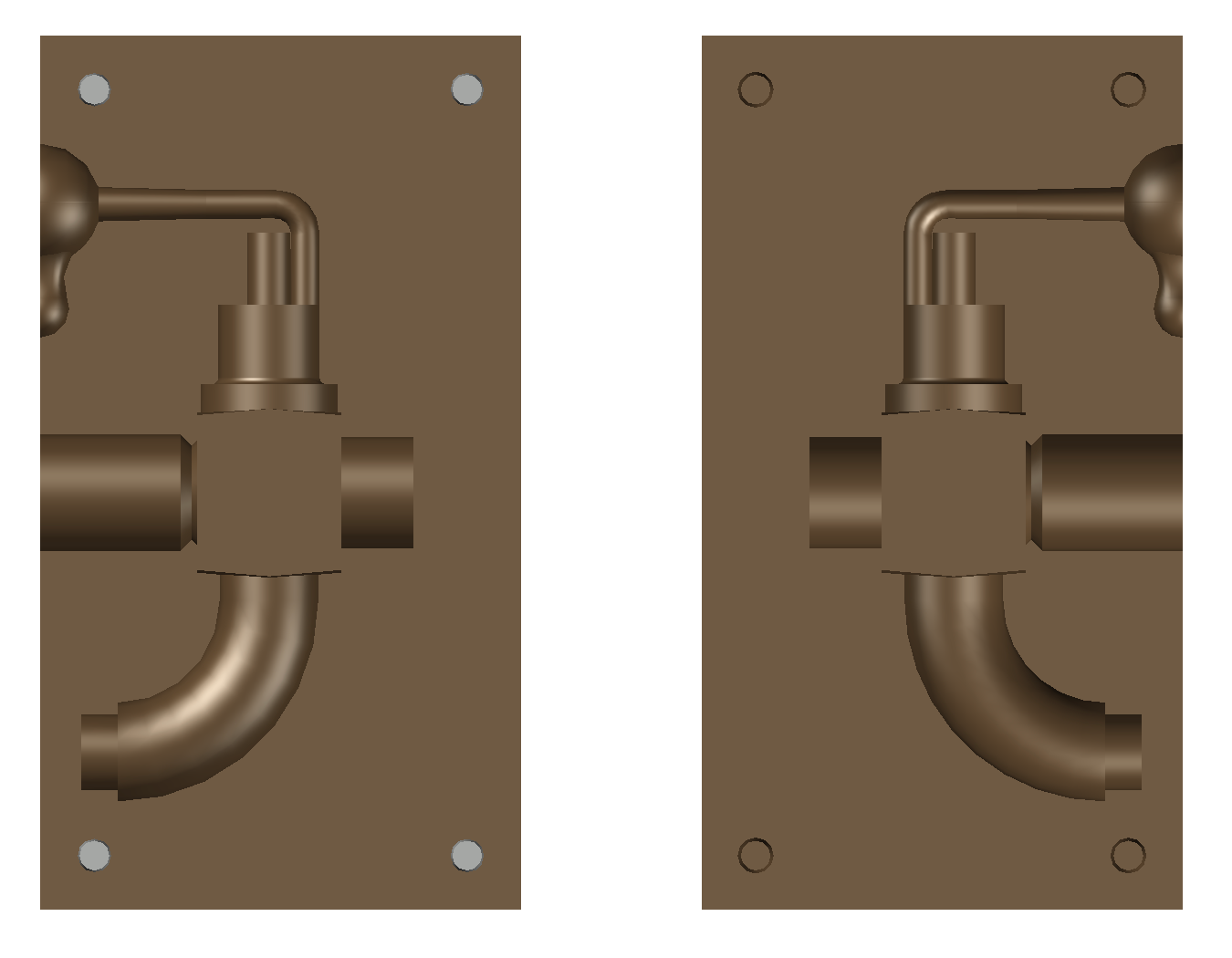
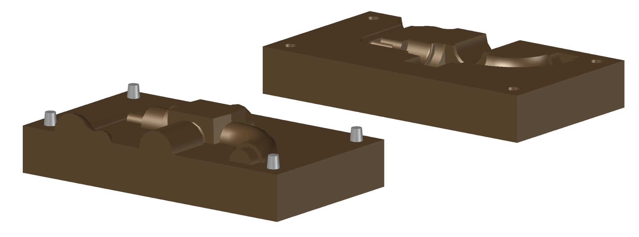
Pattern plate dimensions

The minimum height of the pattern plate must contain the feeder and the neck and the part above the part plus a height below the part of about 15 mm.

Hm=19.5 mm and Lm=2.2 mm

resulting in 55 mm.

This value will be used to dimension the gating system.

The width is equal to the overall dimension plus an allowance of 15 mm on both sides which corresponds to 100 mm.

The thickness of the plate will be equal to 10 mm. pattern plate drawing

Gating system

The aspects to pay attention to in the design of the gating system are listed below:

rapid filling to avoid early solidification;

avoid high velocities;

avoid air entrapment;

block slags;

favorable thermal gradient for directional solidification;

avoid long paths, especially in thin areas.

First of all, you have to choose the type of gating system and indicate the ingates. Since the casting is small, to obtain a favorable thermal gradient, it is sufficient to use a single ingate. For aesthetic reasons, given that the removal of the ingates can leave visible marks on the surface, the outlet side is excluded, which would be preferable for the problems already outlined regarding the feeding distance of the single feeder.

The point chosen in an inconspicuous area, for aesthetic reasons, is shown in the figure.

At this point, the type of gating system must be defined: from the bottom up, from the top or side. For ease of molding, also considering that the shell-molding process was chosen, it is decidedly convenient that the gating system is made along the parting line, therefore the parting line will be vertical.

Placing the sprue in the symmetry and parting plane, there are no constraints on position due to undercut issues.

Sprue

Applying the formulas of Dietert and Nielsen proposed on Santochi

The density of the steel used is 8.0 kg/dm3

Therefore:

Vtot=Vpezzo+Vm=9841.0272 mm3+1401.75 mm3=11251.77 mm3 G=Vtot=8.0 kg/dm30.0112 dm3=0.090 kg

We now calculate the filling time T, using the following formula:

Td=3.2G=0.96 s

considering that the thicknesses b are between 1.5 and 2 mm, repeating the calculation with Nielsen's formula gives:

Tn=3.2bG0.4=2.4 s

the mass flow rate kd and kn calculated respectively with the two formulas: kd=G/Tn=0.0937 kg/s

kn=G/Td=0.0375 kg/s

At this point, the area of the sprue cross-section can be sized, using the formula: S=k/(vel*)

vel is the approximate velocity of the fluid in the section channel, neglecting the pressure drops in the sprue, and is calculated as follows:

considering the dimensions of the pattern plate, the height of the sprue which includes the curvature of the integrated ingate is derived from the height of the pattern plate to the entry point represented in the figure and is equal to:

hc=38.7 mm

vel=2ghc=0.87~m/s

Sd=13.46~mm2 which corresponds to a diameter of 4.14 mm

Sn=5.39~mm2 which corresponds to a diameter of 2.6 mm

Since the height of the free surface below the thread corresponds to about 2.5 mm due to the presence of the machining allowance, the remaining thickness of the order of a millimeter is insufficient to guarantee adequate shell strength. Therefore, it is decided to move the entry point to the tap inlet, exploiting the increased section due to the presence of the machining allowance necessary for subsequent processing, which corresponds to a total thickness of 4 mm.

Setting an ingate diameter equal to 4 mm, the section is 12.56 mm2 which is between the two values Sd and Sn previously calculated.

Since there is only one feeder neck, there is no runner and the section of the feeder neck remains constant. To maintain pressurized flow, the channel is sized following the parabolic law with acceleration due to gravity (ratio between sections inversely proportional to the square root of the heights).

As for the sprue, the textbook Kalpakjian reports that, to avoid air entrapment, the areas of the sections at any two points should follow the law:

A1/A2=h2/h1

For practicality of manufacturing, instead of literally following this (parabolic) law, it is made in a conical shape that still prevents air entrapment at the entrance of the runner, ending with a circular axis section (ingate) of constant section that acts as a choke to keep the flow continuous.

The section is circular for mold release reasons (the parting line is vertical) and manufacturing simplicity. The runner is absent since there is only one ingate. Therefore, the section of the final part of the sprue and of the ingate is constant.

Ingate

The diameter of the ingate is equal to that of the final section of the sprue. It is preceded by a filter. The presence of a slag trap is considered ineffective.

Pouring basin

For the pouring basin, the classic system with two depressions is chosen, one of which receives the beginning of the sprue and where the first slag filter is positioned. The double basin also serves to zero the velocity of the alloy falling from the crucible to respect the design flow velocity at the end of the sprue and thus avoid the risk of turbulence and mold erosion.

The casting is therefore finally the one in the raw casting figure.

Solidification time

According to Chvorinov's rule, with Mp=Vtot/Stot=16607.7268/9722.6078, given a coefficient C equal to 65-70 (for cast irons), with n=2, a time T=1.95 s results.

The values of Vtot and Stot were provided by CAD, therefore they are exact but also considering internal surfaces that have reduced exchange.

Figure of the raw casting

From the calculations performed in the previous sections, the dimensioned geometry of the casting shown in the figure is obtained, where the following are represented: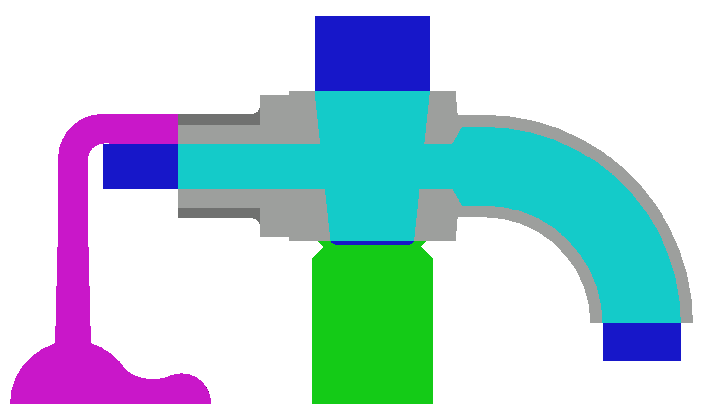

machining allowances

draft angles

fillet radii

feeder

feeder neck

gating system

Subsequent treatments

Once the casting has cooled, the removal of the feeder and the sprue and the removal of any flashes that may have formed along the parting lines or on the contact edges between pattern and core are planned.